Updated August 5, 2023
Introduction to Multicollinearity
Multicollinearity is a phenomenon that occurs when several independent variables in regression progress have high correlation, but not necessarily perfect correlation, with each other.
This can cause unreliable regression results and make it difficult to reject the null hypothesis when it should be rejected. In multiple regression processes, where the impact of changes in multiple independent variables on a single dependent variable is analyzed, several assumptions are made to ensure the validity of the regression results. Upon violation of any of these assumptions, the results become invalid. Multicollinearity is one such violation.

Multiple Regression Equation
A generic form of the multiple regression equation is as follows:
- Y is the dependent variable here.
- b0 is the intercept variable, which represents the value of Y when all independent variables are 0. There is no error term here.
- X1 to Xi are all independent variables, and any change in them impacts the change in Y.
- b1 to bi are the coefficients of the independent variables, sometimes known as the slope coefficients, which determine the magnitude of the change in Y to a change in X.
- Finally, the error term, εi, incorporates the impact on Y that cannot be attributed to a change in any of the independent variables. A good regression equation should have a small error term. This implies that the chosen independent variables can reasonably explain the impact on Y.
Assumptions and Violations of Multiple Regression
To ensure reliable results in Multiple Regression, one must make certain assumptions, violations of which can lead to misleading outputs. In the domain of computer science, this phenomenon is sometimes referred to as GIGO, which stands for Garbage-in-garbage-out. It means that if the input is unreliable or contaminated, the output will also be unreliable or contaminated. The assumptions in Multiple Regression include:
- Dependent variable Y and independent variables X1…Xi is linearly related.
- The independent variables X1…Xi is not random, and no linear relationship exists between any of them. The violation of this assumption is multicollinearity.
- The expected value of the error terms associated with each independent variable is 0, which enables us to be reasonably sure that the independent variable is a good indicator of the dependent variable.
- The variance of the Error term is the same for all observations (Homoskedasticity), and the violation of this assumption is what we know as Heteroskedasticity.
- Error terms are not correlated, and the violation is called Serial correlation.
- The error term has a normal distribution.
It is important to note that these are the assumptions of multiple regression, and violations of other assumptions are also part of statistical theory and are studied in great detail. However, the focus of this article is on the violation of one specific assumption.
Impact of Multicollinearity
During the process of coming to a regression output, one engages in hypothesis testing, formulating a Null Hypothesis (H0) and an Alternate Hypothesis (Ha). The Null Hypothesis generally represents the opposite of the desired result, and the goal is to reject it through the regression process. The Alternate Hypothesis, on the other hand, encompasses the desired result and is automatically proven when the Null Hypothesis is rejected.
However, when multicollinearity exists, one is unable to reject the Null Hypothesis, which would have been possible in the absence of multicollinearity. Therefore, one cannot confidently conclude that the regression process is valid or meaningful.
Detection of Multicollinearity
To determine if multicollinearity exists, it is necessary to identify any anomalies in our regression output. The steps to reach this conclusion are as follows:
1. R2 is High
R2, also known as the coefficient of determination, is the degree of variation in Y that can be explained by the X variables. Therefore, a higher R2 value indicates that a significant amount of variation is explained through the regression model. In multiple regression, one uses the adjusted R2, which one derives from the R2 but is a better indicator of the regression’s predictive power as it determines the appropriate number of independent variables for the model. Despite a high adjusted R2, if we conclude that the regression is not meaningful, then one can suspect the presence of multicollinearity.
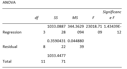
2. F–stat is Significant
This test functions to reject the null hypothesis, which states that all slope coefficients in the regression equation are equal to 0. If this statistic is significant, one can safely reject the null hypothesis and conclude that at least one slope coefficient is not equal to 0. Therefore, a change in one or more X variables can explain some part of the change in Y. One of the indicators of multicollinearity is a highly significant F-stat, even though the regression model may not have good predictive power.
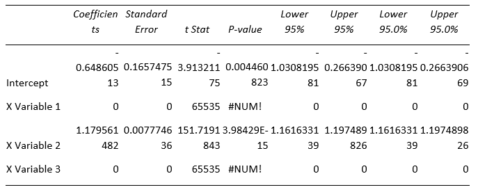
3. T–stat is Insignificant
If the first two points are true, one examines the T-stat of each X variable. If the T-stat is insignificant, and one is unable to reject the null hypothesis, one should check for multicollinearity. We set up a Null Hypothesis for the slope coefficient of each X variable. If one believes the coefficient should be negative, one has the following one-tailed T-test Hypotheses:
- H0: bi ≥ 0
- Ha: bi < 0
4. T–stat = bi – 0 / Standard Error
bi is the predicted value of the slope coefficient, and 0 is the hypothesized value.
One assumes a certain significance level and compares the T-stat to the critical value at that level, and then comes to the conclusion of whether the slope coefficient is significant or not. If it is insignificant, then one can conclude the presence of multicollinearity.
In cases of multicollinearity, the standard errors become unnaturally inflated. This can lead to the inability to reject the null hypothesis for the T-stat. Certain software packages provide a measure for multicollinearity known as the VIF (Variance Inflation Factor), where a VIF value greater than 5 suggests high multicollinearity.
Example of Multicollinearity (With Excel Template)
Below are some examples of implementing multicollinearity:
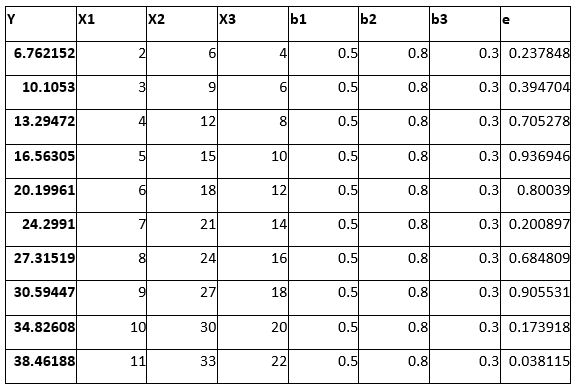
- Here, as one can see, X2 = 3 × X1 and X3 = 2 × X1. Thus, all the independent variables correlate as per the definition of multicollinearity,
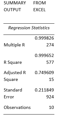
- However, producing a regression output using Excel gives num error, as this dataset contains a violation of regression assumptions i.e., multicollinearity. It means that Excel cannot calculate the regression for an input that contains a violation. Other software packages contain different calculation methods, for instance, VIF. Therefore, they can run a regression with data containing multicollinearity.
Conclusion
One way to mitigate the effects of multicollinearity is to omit one or more independent variables and observe the impact on the regression output. However, it is important to note that multicollinearity cannot be completely eliminated. In real-world scenarios, the factors affecting a dependent variable are often somewhat correlated. At best, we can only consider the degree of correlation and take appropriate measures accordingly. In general, a low degree of correlation among independent variables is preferable. This avoids potential issues with multicollinearity in regression analysis.
Recommended Articles
Here are some further articles for expanding understanding: