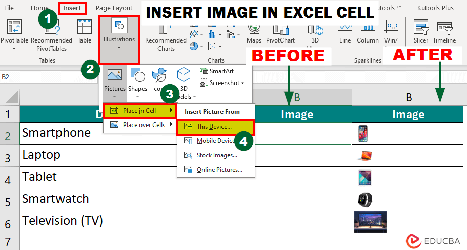
How to Insert Image in Excel Cell?
While Excel is primarily known for its numerical and text-based functions, we can also insert images into Excel cells. This makes Excel a more valuable tool, as incorporating images can add depth and clarity to your spreadsheets and enhance visual presentations, data analysis, and reports.
Using this detailed step-by-step guide, you can easily learn how to insert image in Excel cells.
Table of Contents
- How to Insert Image in Excel Cell?
- 4 Easy Methods to Insert Image/Picture in Excel (Stepwise Guide)
- How to Lock and Resize Images in Excel Cell?
4 Easy Methods to Insert Image/Picture in Excel (Stepwise Guide)
We will see the following methods to insert image in Excel cells in this article.
- Place in Cell
- Place over Cells
- Using IMAGE Function
- Using VLOOKUP, INDEX & MATCH Functions
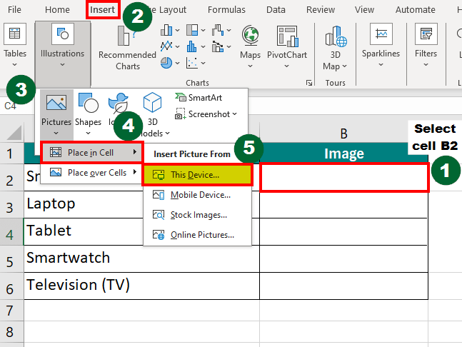
Method 1: Place in Cell
Follow these instructions to use the place in cell option:
1. Select the cell (e.g., cell B2) where you want to place the picture.
2. Go to the “Insert” tab at the top of the window.
3. Click on the “Pictures” option present under the “Illustrations” group.
4. Select “Place in Cell.”
5. Then, select the location from where you want to add the picture. We have chosen “This Device” as we downloaded a few images online.
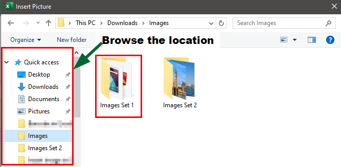
6. Find the image file on your computer.
7. Choose the image and click the “Insert” button.
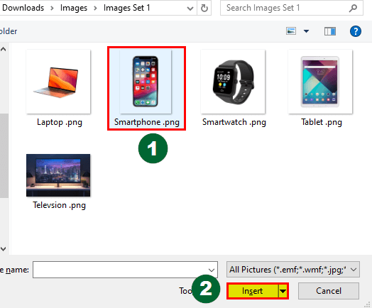
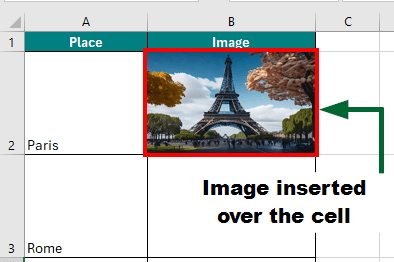
The selected Image is Inserted in the particular cell, i.e., cell B2.
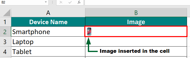
To preview the image, you can select cell B2 and Press Ctrl+Shift+F5.
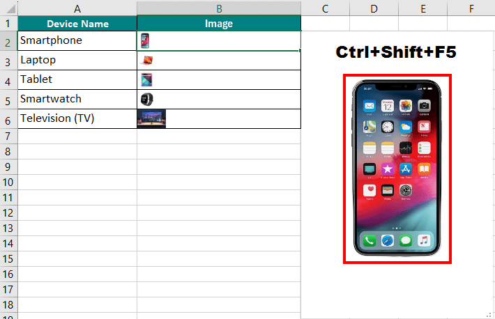
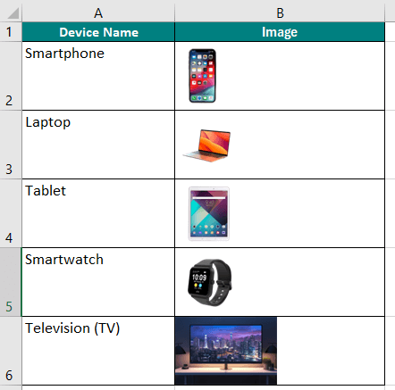
Similarly, you can insert the rest of the images and adjust the row height and column width for proper visuals.
Method 2: Place over Cells
- Select cell B2.
- Go to the “Insert” tab.
- Click the “Illustrations” group.
- Select the “Pictures” option.
- Choose “Place over Cells,” and select your preferred option. For instance, we have chosen “This Device”.
- Find the image file on your computer.
- Choose the image and click the “Insert” button.
To resize the image to fit in the particular cell, right-click the image and select “Format Picture”.
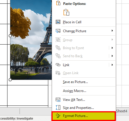
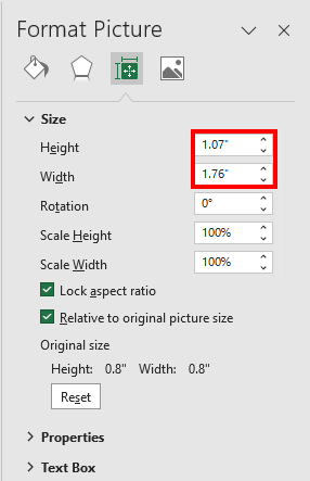
A dialog box will appear in which you can select size & properties and adjust the height and width of the image.
Method 3: Using IMAGE Function
While using the IMAGE function, you can follow two approaches, as shown below.
A) Directly add the image address in the IMAGE Function
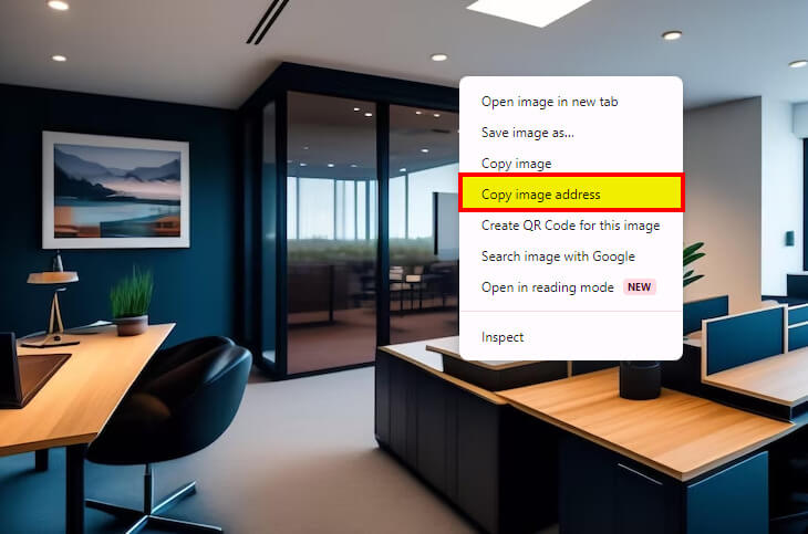
Copy the address of the image that you want to insert by right-clicking on the image and selecting “Copy image address.” You can use images from Google or any free image website.
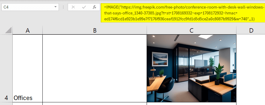
In your preferred cell, for instance, Cell C4, add the image formula:
that-says-office_1340-37385.jpg?t=st=1708169332~exp=1708172932~hmac=
ed174f6cd1e923b1e99e7f7176f936ceaf1912fcc9fd1d5d5ce2a0c8087b9929&w=740”,,1)
The above formula has this simple syntax: =IMAGE(source, [alt_text], [sizing], [height], [width])
- source: This is the URL of the image you want to insert
- alt text: Description of the image. Optional.
- sizing:
- 0: Fit the image in the cell while maintaining the picture’s original aspect ratio.
- 1: Fit the image in the cell, ignoring the picture’s original aspect ratio.
- 2: Maintain the original image size, which may exceed the cell boundaries.
- 3: Customize image size using height and width arguments.
- height: Custom height of the image in pixels. Optional.
- width: Custom width of the image in pixels. Optional.
We have inserted the copied image address where it says “Source,” replaced “Sizing” with “1” in the formula, and left the optional arguments like Alt text, Height, and Width blank.
After that, press enter, and Excel will display the image in the designated cell.
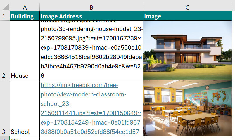
B) Add image address as cell reference in IMAGE Function
Let’s say you already have a list of image addresses (URLs) in column B, and you want to display the images in column C. To do this, you can use the IMAGE function in this manner:
Assuming that the image address is in cell B2, type the following formula in cell C2:
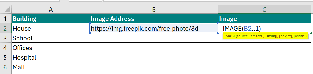
This will add the image address present in cell B2 as the source (URL of the image you want to insert), and the IMAGE function will display the corresponding image.
Method 4: Using VLOOKUP, INDEX & MATCH Functions
As of now, we have seen how to insert a single image/picture in an Excel cell. Now, let us see how you can create a dashboard with a dynamic Excel cell. It means if you change the location name in your dashboard, Excel will automatically replace the old image and update a new image. We can do this using lookup Formulas like VLOOKUP, INDEX, and MATCH.
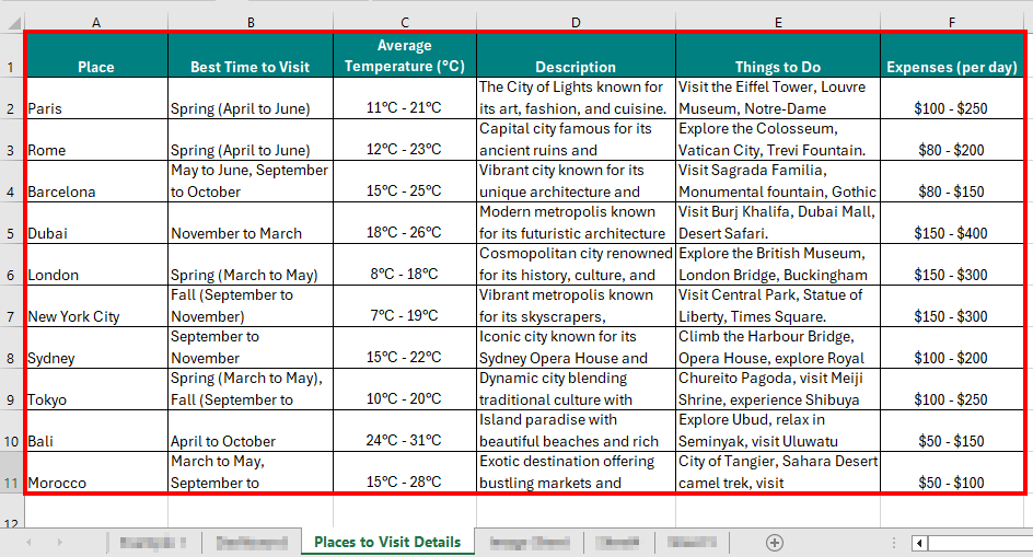
For this, suppose in the sheet “Places to Visit Details,” we have a list of places to visit with a few details like:
- Place Name
- Best Time to Visit
- Average Temperature
- Description
- Things to Do
- Expenses Per Day
Follow these steps to insert images dynamically in Excel cells.
Step 1: Create a new sheet named “Dashboard” and enter all details.
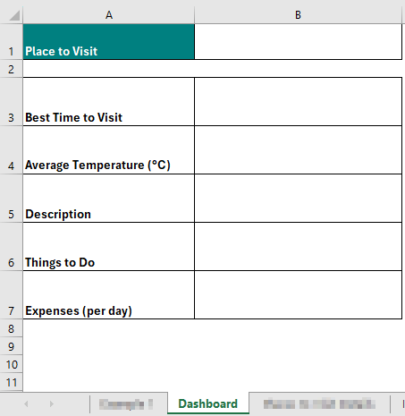
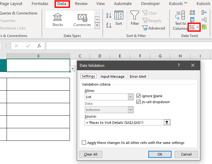
Step 2: To add the list of places as a dropdown menu,
- Select cell B1.
- Go to the “Data” tab.
- Click on “Data Validation” from “Data Tools”.
- Create a list of all the places’ names by adding cell reference (=’Places to Visit Details’!$A$2:$A$11) in the source textbox.
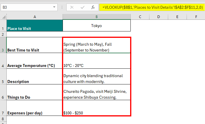
Step 3: To display all the details of the selected place, add the below VLOOKUP Formula in cells B3 to B7:
This will get details for ”Best Time to Visit,” “Average Temperature (°C),” “Description”, “Things to Do,” and “Expenses (per day).”
Step 4: Now, to display the respective image of the selected place, we will first need to create a named range. You can do that by following the given steps:
- Go to the “Formulas” tab.
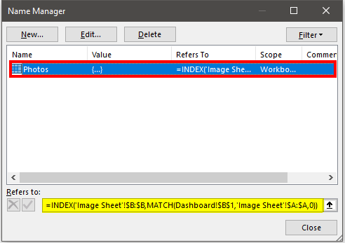
- Under the “Defined Names” group, select “Define Name” or click on “Name Manager.” This will open the “Name Manager” window.
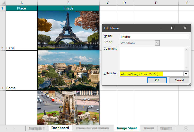
- In the “New Name” dialog box, enter a name. Let’s call it “Photos” for this example.
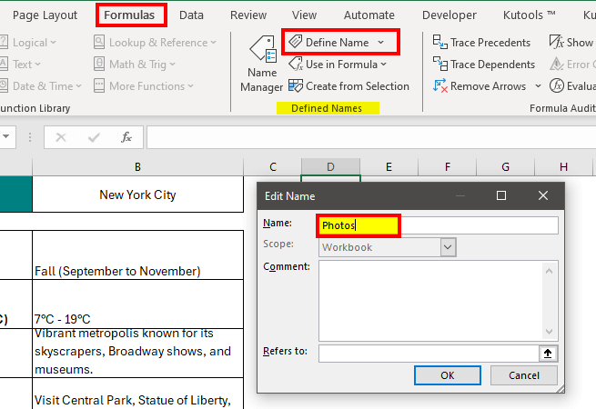
- Next, enter the below INDEX formula in the “Refers to” field:
In this case, we have added the whole B column from the “Image Sheet” as an array.
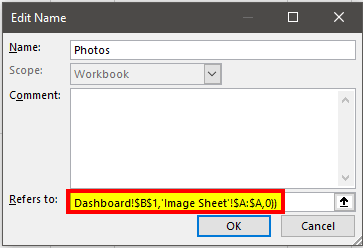
- Then, after the comma, type the below MATCH function formula:
Here, we first selected the “Place to Visit Name,” i.e., cell B1 from the “Dashboard” Sheet. Then, we added the entire first column, i.e., “Place name” from the “Image Sheet.” Next, we entered “0” to specify that we need an exact match. Finally, we close the INDEX and MATCH functions using two closing brackets.
Step 5: Click “OK” to save the named range.
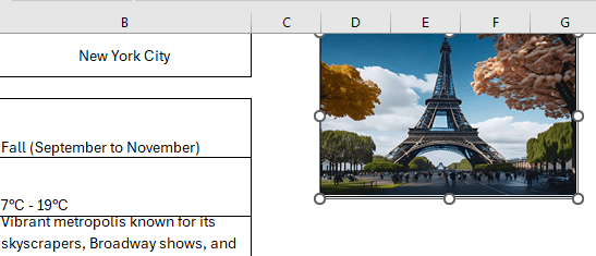
Step 6: Now, we need to select a cell in the dashboard sheet where we want the image to be displayed. For this, you can simply:
- Go to the “Image” sheet and copy any cell where an image is present.
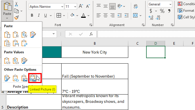
- Then go to the “Dashboard” sheet and select the cell where you want to paste the linked picture.
- In the “Home” tab, choose “Paste Special“.
- In the “Paste Special” dialog box, select “Linked Picture” and click “OK“.
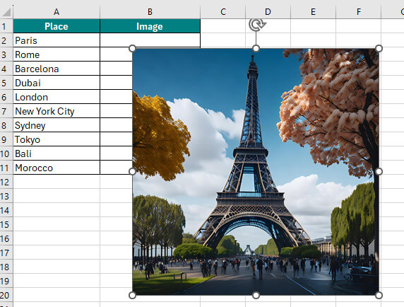
You will now see the image pasted onto the “Dashboard” Sheet as a linked picture.
Step 7: To display the correct image based on the selected place name, follow these steps:
- Click on the linked picture.
- In the formula bar at the top, you will see the cell reference (=’Image Sheet’!$B$2) of the linked picture.
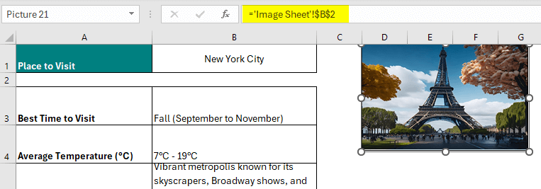
- Replace the cell reference with the name of the named range you created earlier (“Photos” in this example).
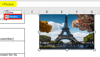
Step 8:
- Press Enter.
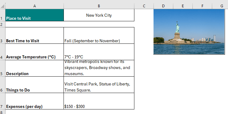
Now, whenever you select a place name from the dropdown in the “Dashboard” Sheet, the linked picture will change accordingly, displaying the palace photo from the “Image Sheet.”
How to Lock and Resize Images in Excel Cell?
A) To Resize:
Let’s say you have added more than one image in Excel cells and want to resize all images at once.
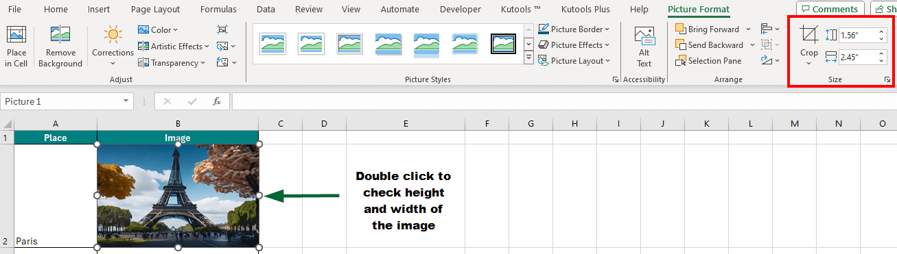
1. First, You must ensure that the edges of all the added images are aligned with the cell’s borders. You can also check the height and width of the image by double-clicking on the image.
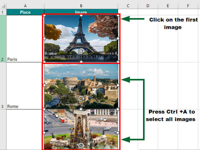
2. Once done, select all the images in the active worksheet by clicking on the first image and then press “Ctrl + A“.
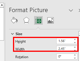
3. After selecting all the images, press “Ctrl + 1” to open the “Format Picture” dialog box. Under which, you can select “Size & Properties” and adjust the size of all images as required.
B) To Lock:
By “locking” the picture to the cell, you essentially tell Excel to treat the image as part of the cell’s content. So, if you move, filter, or hide the cell, the picture will also move, filter, or hide along with it. This helps to maintain the relationship between the image and the cell, keeping your spreadsheet organized and readable.
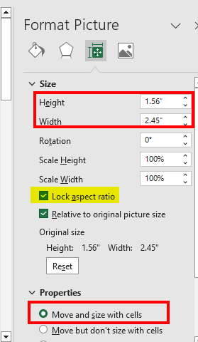
5. After setting the required height and width, you must select the “Lock aspect ratio” option to keep the images locked in their respective cells.
6. Then, under the Properties tab, check the “Move and size with cells” option to ensure the picture is locked to the cell. As a result, as the cell size changes, the image size will also change.
Recommended Articles
We hope you liked our guide on inserting images in Excel Cell! This guide discussed inserting an image in Excel using place-in-cell and place-over-cell options. We also showed you how to add an image in an Excel cell using IMAGE, VLOOKUP, INDEX and MATCH functions. If you found this guide helpful, you can also explore some of the other useful articles:
