Introduction to VLOOKUP Examples in Excel
This article covers one of the most helpful features, which is VLOOKUP. Simultaneously it is one of the most complex and less understood functions. This article will demystify VLOOKUP with a few examples(VLOOKUP Examples in Excel).
Examples of VLOOKUP in Excel
VLOOKUP in Excel is very simple and easy to use. Let’s understand how to use the VLOOKUP in Excel with some examples.
Example #1 – Exact Match (False or 0)
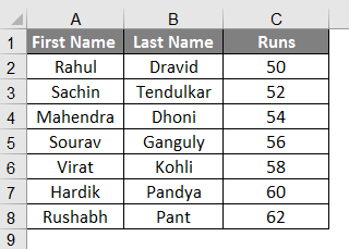
Here for this example, let’s make a table to use this formula; suppose we have the data of students as shown in the image below.
In cell F2, we are using VLOOKUP Formula. We have made the table; by using Vlookup, we will find the person’s Last name from their first name; all the data has to be available in the table, which we are providing the range to find the answer within (A: C in this case).
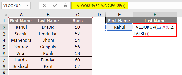
- We can select the table instead of the entire row; In the formula, you can see written 2 before False as a column indicator because we want data to be retrieved from column # 2 from the selected range.
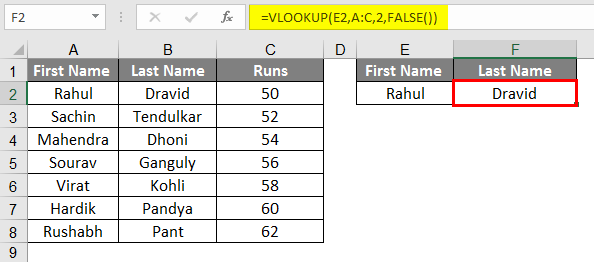
- When we place data in E3, the first name from our given table, the formula will give us the Last Name.
- When we enter the first name from a table, we are supposed to get the formula’s last name.
- From the Image above, we can see that by writing the name Rahul in the column, we got Dravid as the second name, according
- to the table on the left.
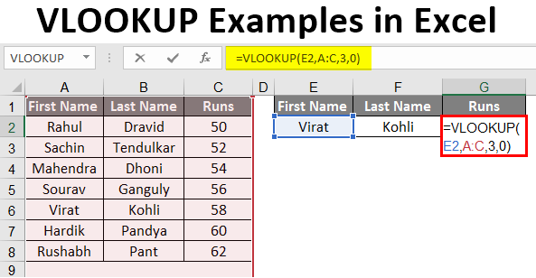
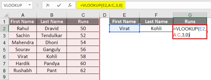
- Now we can also widen the data from a single data available, so by just filling in the First Name, we will have the Last name of the person and the runs scored by that person.
- So let’s add the third column on the right side, “Runs”.
- After applying VLOOKUP Formula, the result is shown below.
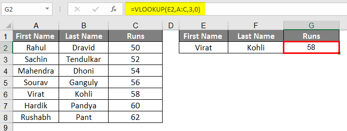
- We can see that just from the first name, we have the last name and the runs scored by that student; If we retrieve runs from the last name column, it will be called chained Vlookup.
- Here you can see we have written 3 as we want the data of column #3 from the range we have selected.
- Here we have used False OR 0, which means it matches the absolute value, so by applying even extra space to our first name, it will show the #N/A means data not matching.
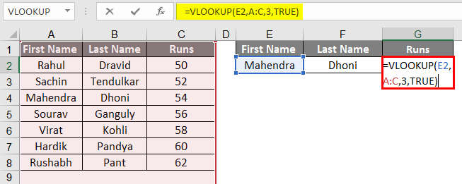
Example #2 – Approximate Match (True or 1)
- If we apply the same formula with True or 1 instead of False or 0, we will not have to worry about providing the exact data to the system.
- This formula will provide the same results, but it will start looking from top to bottom and provide the value with the most approximate match.
- So even after you make a spelling mistake or a grammatical error, in our case, you don’t need to worry, as it will find the most matched data and provide the mostly matched result.
- After applying VLOOKUP Formula, the results are shown below.
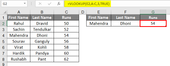
- In our example, we have written Mahendra in the first name, and we are still getting the result correctly; this can be a bit complicated while you’re playing with the words, but you are more comfortable working with Numbers.
- Suppose we have Numeric data instead of the name, word, or alphabetical; we can do this more precisely and with more authentic logic.
- It seems pretty useless as we are dealing with small data here, but it is very useful while dealing with large data.
Example #3 – Vlookup from a Different Sheet
- Vlookup from a different sheet is very similar to the Vlookup from the same sheet, so here we have changed the ranges and have different worksheets.
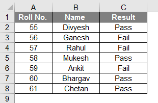
- We have a table in sheet number 2 as per the following image; we will find the result of this student in sheet number 3 from their roll nos.
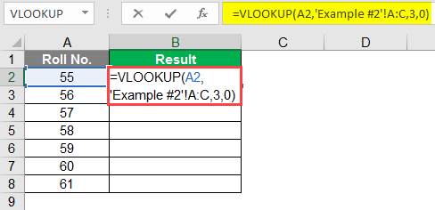
- As you can see, the image on the right side is of another sheet, sheet number 3.
- Apply the VLOOKUP Formula in Column B.
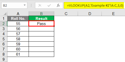
- After applying VLOOKUP Formula, the result is shown below.
- Drag down the formula for the next cell. So the output will be as below.
- From the above images, you can see that the range of the formula has been indicated with ‘Example#2′ as the data we needed will be retrieved from Example #2 and column #3. So as a column indicator, we have written 3, and then 0 means False as we want an exact data match.
- As you can see from the below image, we have successfully retired the entire data from Example #2 to Sheet # 3.
- You can see from the above image after getting the value in the first row; we can drag the same and get to throughout data against the given roll nos if it is available in the given table.
Example #4 – Class Using Approx Match
- To define class from the marks, we can use an approx match to define the class against the Marks.
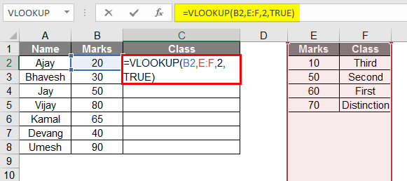
After using the VLOOKUP formula, the result is shown below
- As per the above image, you can see that we have made a table of students with marks to identify their class; we have made another table that will act as the key,
- But make sure that the marks in the cell have to be in ascending order.
- So in the given data, the formula converts the marks into a grade from the class table or “Key” table.
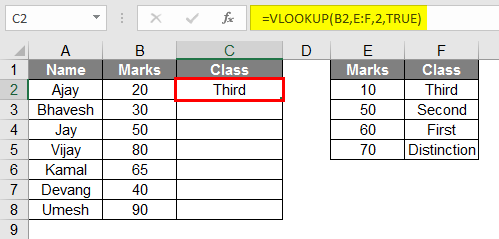
- Drag the same formula from cell C2 to C9.
Example #5 – Dual Lookup Using Match function
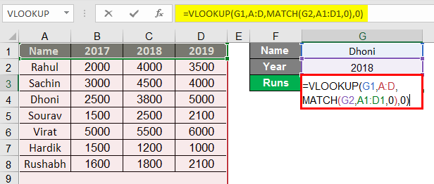
- The Match function is used when we need to look up two-way data; here, from the above table, you can see data of batsmen against the runs they scored in particular years.
- So the formula to use this match function is as follows:
=vlookup(lookup_Val, table, MATCH(col_name, col_headers,0),0)
- After applying the Formula, the result is shown below.
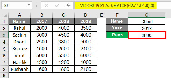
- Here if we study the formula, we can see that our data is dependent on two data; in our case, what we write in G1 and G2, in the Match function, we have to select the Column Headers, any of the headers have to be written in G2 which is dedicated to the column name.
- In column G1, we must write the data from the Row of the player’s Name.
- The formula becomes as follows:
=vlookup(G1, A:D, MATCH(G2, A1:D1,0),0)
- In the given formula, MATCH(G2, A1:D1,0) is selected column header cell G2 has to be filled by one of the headers from the selected column header.
- It returns that Dhoni scored 3800 Runs in 2018.
Recommended Articles
This is a guide to VLOOKUP Examples in Excel. We discuss using VLOOKUP in Excel, some practical examples, and a downloadable Excel template. You can also go through our other suggested articles –
