Updated August 10, 2023
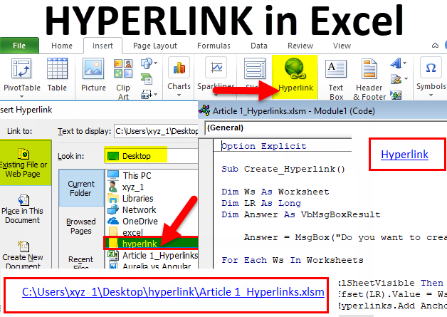
Introduction to HYPERLINK in Excel
HYPERLINK in Excel allows users to create a shortcut to reach any worksheet, file, folder, or webpage. It helps us to reach any specific folder or link quickly.
We also use hyperlinks to provide references. The hyperlinks option is in the Insert menu option under the Links section. We have to provide the text on which we want a hyperlink and then select the file or website page we want to link with that text.
So, HYPERLINK creates a link to cells, sheets, and workbooks.
Where to Find Hyperlink Option in Excel?
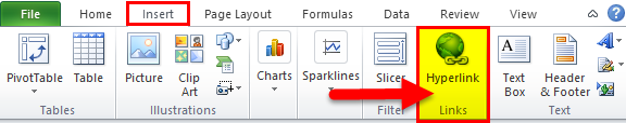
In Excel, a hyperlink is located under Insert Tab. Go to Insert > Links > Hyperlink.
This is the rare use path. About 95% of the users do not even bother going to the Insert tab to find the Hyperlink option. They rely on the shortcut key.
The shortcut key to open the Hyperlink dialogue box is Ctrl + K.
How to Create HYPERLINK in Excel?
HYPERLINK in Excel is very simple and easy to create. Let’s understand how to create HYPERLINK in Excel with some Examples.
Example #1 – Create a Hyperlink to Open Specific File
Ok, I will go one by one. I am creating a Hyperlink to open the workbook I use very often when creating reports.
I cannot keep going back to the file folder and clicking to open the workbook; rather, I can create a hyperlink to do the job.
Step 1: Press Ctrl + K. (Shortcut to open the hyperlink) in the active sheet. This will open the below dialogue box.
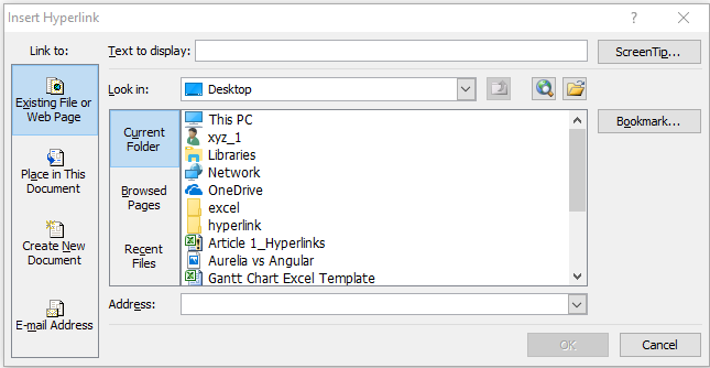
Step 2: There are many things involved in this hyperlink dialogue box.
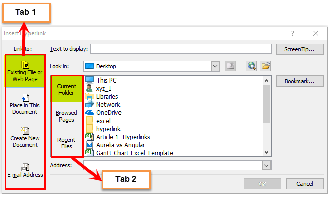
Mainly there are two tabs available here. In Tab 1, we have 4 options, and in Tab 2, we have 3 options.
Step 3: Go to the Existing File or Web Page. (By default, when you open a hyperlink, it has already been selected)
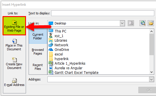
Step 4: Select Look in Option. Select the location of your targeted file. In my case, I have selected Desktop and in the desktop Hyperlink folder.
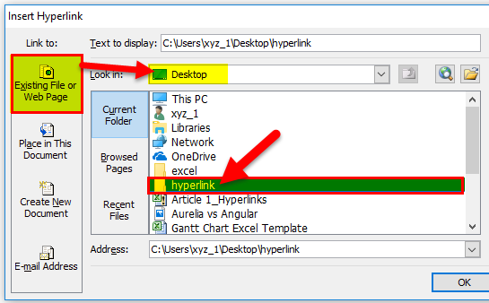
Step 5: If you click on the specified folder, it will show all the files stored in it. I have a total of 2 files in it.
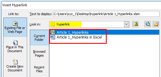
Step 6: Select the files that you want to open quite often. I have selected the Article 1_hyperlinks file. Once the file is selected, click on Ok. It will create a hyperlink.
Initially, it will create a hyperlink like this.
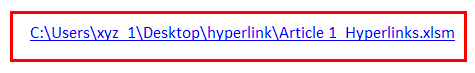
Step 7: Now, for our understanding, we can give any name to it. I am only giving the name as the file name, i.e., the Sales 2018 file.

Step 8: if you click on this link, it will open up the linked file. In my case, it will open the Sale 2018 file on the Desktop.
Example #2 – Create a Hyperlink to Go to a Specific Cell
Now we know how to open a specific file by creating a hyperlink. We can go to the particular cell as well.
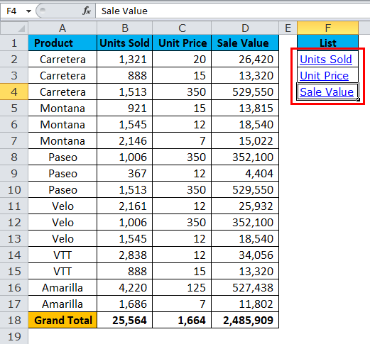
I have a product list with their quantities sold, unit price, and sales value. At the end of the data, I have a total for all these 3 headings.
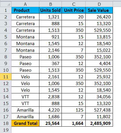
Now, if I want to keep going to the Unit Sold total (B18), Unit Price Total(C18), and Sales Value (D18) total, it will be a lot of irritating tasks. I can create a hyperlink to these cells.
Step 1: Create a List.
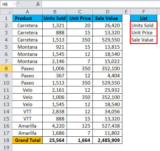
Step 2: Select the first list, i.e., Units Sold, and press Ctrl + K. Select Place in this Document and Sheet Name. Click on the Ok button.
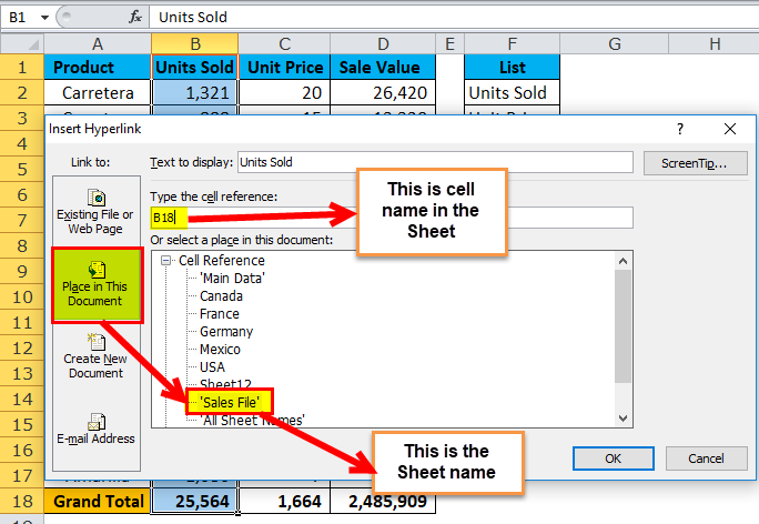
Step 3: It will create the hyperlink to cell B18.
If you click on Units Sold (F2), it will take you to cell B18.
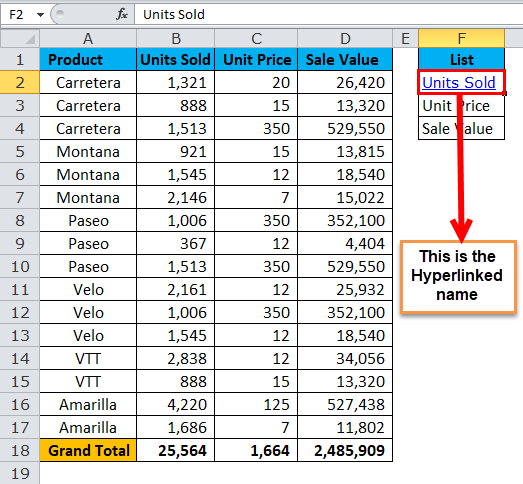
Step 4: Select the other two cells and follow the same procedure. Finally, your links will look like this.
Units Sold will take you to B18.
Unit Price will take you to C18.
The sale Value will take you to D18.
Example #3 – Create Hyperlink to Work Sheets
As I mentioned at the start of this article, if we have 20 sheets, it is very difficult to find the sheet we want. Using the hyperlink option, we can create a link to those sheets, and with just a click of the mouse, we can reach the sheet we want.
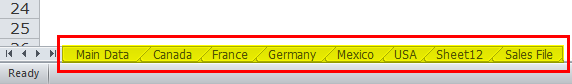
I have a total of 8 sheets in this example.
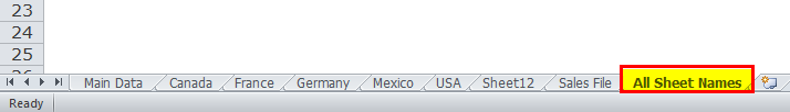
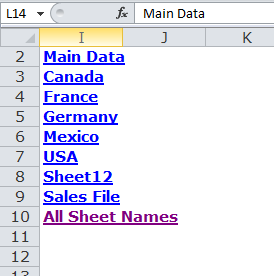
Step 1: Insert one new sheet and name it All Sheet Names.
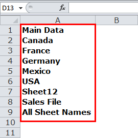
Step 2: Write down all the sheet names.
Step 3: Select the first sheet name cell, i.e., Main Data, and press Ctrl + K.
Step 4: Select Place in this Document > Sheet Name.
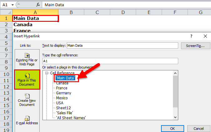
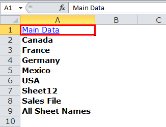
Step 5: This will create a link to the sheet name called Main Data.
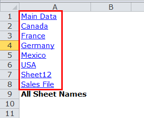
Step 6: Select every one of the sheet names and create the hyperlink.
Step 7: Now, for our understanding, we can give any name to it. I am only giving the name as the file name, i.e., the Sales 2018 file.
Create Hyperlink Through VBA Code
Creating Hyperlinks seems easy, but if I have 100 sheets, it isn’t easy to create a hyperlink for each one.
Using VBA code, we can create the entire sheet hyperlink by clicking on the mouse.
Copy and paste the below code into the Excel file.
Go to Excel File > Press ALT + F11 > Insert > Module > Paste
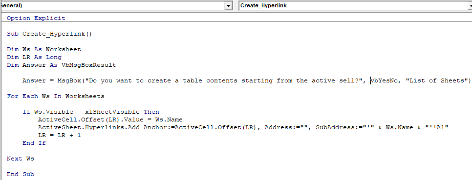
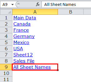
This will create hyperlinks and a list of all the sheet names in the workbook.
Things to Remember About HYPERLINK in Excel
- We can create a hyperlink by using the HYPERLINK function.
- We can create a hyperlink to open any file within the same computer.
- We can give any name to our hyperlink. In the case of hyperlinking worksheets, it is not mandatory to mention the same name in the hyperlink.
- Always use VBA code to create a hyperlink. Because whenever there is an addition to the worksheet, you have to run the code, which automatically creates a hyperlink for you.
- We can go to the specified cell, specified worksheet, and established workbook using hyperlinks. It will save a lot of our time.
Recommended Articles
This has been a guide to HYPERLINK in Excel. We discuss its uses and how to create HYPERLINK in Excel with Excel examples and downloadable Excel templates. You may also look at these useful functions in Excel –
