Updated July 5, 2023
Heat Map in Excel
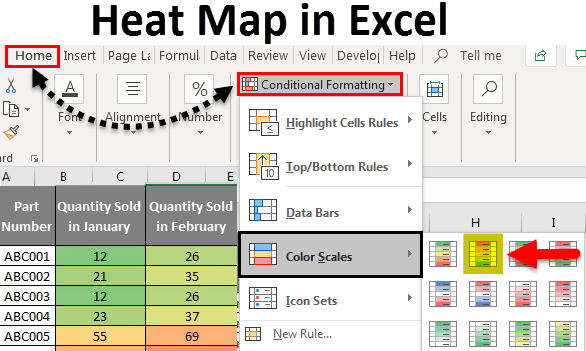
Heat Map in Excel is used to show data in different color patterns. In Heat Map, data is shown in a different color pattern to see which data point is below the limit and which is above the limit. In addition, we can use two or more two colors to see the data pattern.
This helps in judging whether the data target is achieved or not.
How to Create a Heat Map in Excel?
Instead of manual work, conditional formatting can highlight value-based cells. If you change the values in the cells, the color or format of the cell will automatically update the heat map in conditional formatting based on the predefined rules.
Let’s understand how to Create a Heat Map in Excel by using some examples.
Example #1
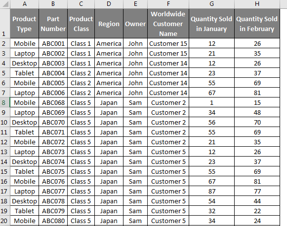
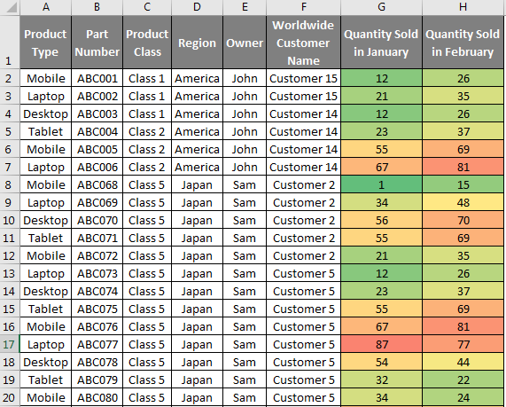
Here we got the sales data of some part numbers. Where we have the sales numbers in Columns G and H for two months. Now we want to apply Heat maps to the data shown below.
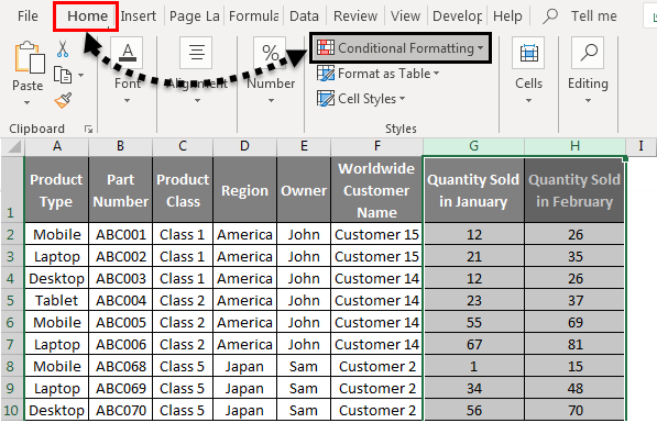
For that, first, select both columns, G and H. Now go to the Home menu and select Conditional Formatting, as shown below.
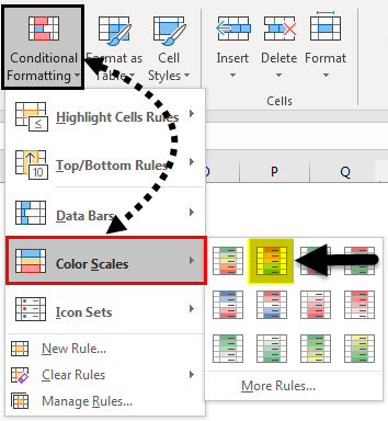
Once we do that, we will get a drop-down menu list, as shown below. Now from Color Scales, select any color pattern. We have selected the second option, the Red-Yellow-Green color pattern, as shown below.
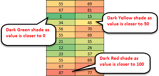
Once we do that, we will see the heat pattern for all selected color scales, as shown below. This shows that the value less than 50 is in green color shades. The mid-value, near to 50, is in yellow shades, and the value, near to 100, is in red shades.
Values closer to the limit have dark shades, and the values far from the limit have light shades. Let’s see a small patch of data and measure the different color scale values, as shown below.
So this is how the color scaling can be done for Heat maps in any data. We can choose different color scaling as well as per our color choice.
Example #2
There is another method of creating a Heat Map in Excel. This is an advanced method of creating heat maps with more features. Select columns G and H and follow the same path discussed in the above example.
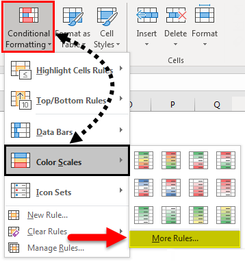
- Go to the Home menu, and click on Conditional Formatting. Once we do that, we will get a drop-down list of it.
- Then click on Color Scales from the side list and select More Rules, as shown in the below screenshot.
This will take us to the advanced option of Formatting Rules for Heat Maps through Conditional Formatting. It will open the New Formatting Rule window, as shown below.
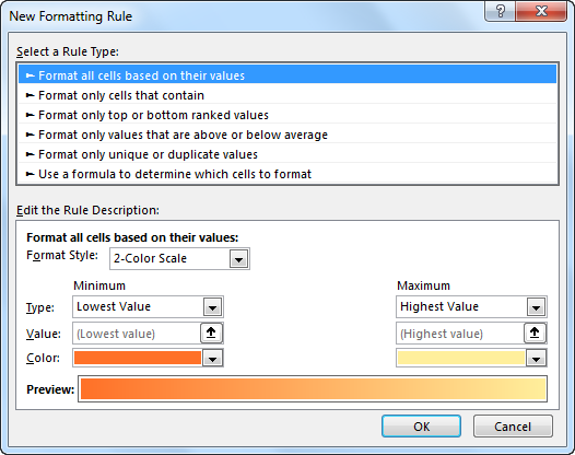
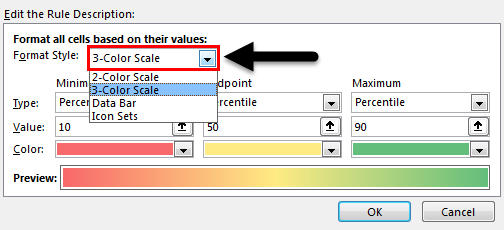
For the selected data set, let’s create a new rule for the heat map. We can create a new rule or go ahead with existing rules. As we can see, in Edit the Rule Description box, a Format Style tab is available with a drop-down button. Select the 3 Color Scale as shown below.
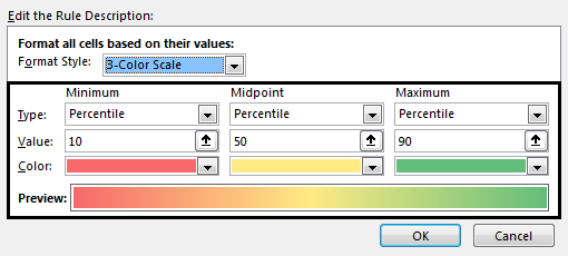
Once we do that, we will see the 3 different color scales with a value range, as shown below. Here, all 3 colors have the default value set in them.
Now for the complete range, Minimum, Midpoint, and Maximum, select the range by clicking on an icon![]() , or we can write the number we need to see the Heat Map color scaling. And click on OK. As shown below, we have chosen 0 as the Minimum percentile range, 50 as the Midpoint percentile range, and 100 as the Maximum percentile range.
, or we can write the number we need to see the Heat Map color scaling. And click on OK. As shown below, we have chosen 0 as the Minimum percentile range, 50 as the Midpoint percentile range, and 100 as the Maximum percentile range.
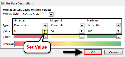
Note: We can change the color from the below color tab and check the preview for the color scaling.
Once we click OK, we will get the heat map created for the selected data set, as shown below.
As we can see above, with the help of selected color scaling, we got the Heat Map created, which shows higher the data, the dark will be the red color, and the lower the data, the more light will be the green color. And Midpoint data is also showing the color change concerning the defined or selected value range. Here for the selected Midpoint value 50, data is changing color to and fro.
Pros
- For a huge set of data where applying a filter will not give the actual picture of data changes. If we create Heat Map, we can see the change in value without applying the filters.
- For the data where we need to see the area (Region, Country, City, etc.) wise changes, in this case, using Heat Map gives high and safe points in the selected color scale.
- It is always recommended to use Heat Map when the data size is huge and the data pattern fluctuates at some specific points.
Cons
- It is not advised to keep any Conditional Formatting function applied in data for a long time because it makes Excel work slow while we use the filter to sort the data.
Things to Remember About Heat Map in Excel
- Always clear the conditional formatting rule once its use is done. Or else save the rule so that it can be used later.
- Choose color scales with Heat pattern that are easy to show and measure.
- Measure the range before selecting, and fix the scaling points so that colors and data points can be fixed above and below those values.
Recommended Articles
This has been a guide to Heat Map in Excel. Here we discussed How to create Heat Map, practical examples, and a downloadable Excel template. You can also go through our other suggested articles–
