Updated March 20, 2023
What is GLM in R?
GLM in R is a class of regression models that supports non-normal distributions and can be implemented in R through glm() function that takes various parameters, and allowing user to apply various regression models like logistic, poission etc., and that the model works well with a variable which depicts a non-constant variance, with three important components viz. random, systematic, and link component making the GLM model, and R programming allowing seamless flexibility to the user in the implementation of the concept.
GLM Function
Syntax: glm (formula, family, data, weights, subset, Start=null, model=TRUE,method=””…)
Here Family types (include model types) includes binomial, Poisson, Gaussian, gamma, quasi. Each distribution performs a different usage and can be used in either classification and prediction. And when the model is gaussian, the response should be a real integer.
And when the model is binomial, the response should be classes with binary values.
And when the model is Poisson, the response should be non-negative with a numeric value.
And when the model is gamma, the response should be a positive numeric value.
glm.fit() – To fit a model
Lrfit() – denotes logistic regression fit.
update()- helps in updating a model.
anova() – its an optional test.
How to Create GLM in R?
Here we shall see how to create an easy generalized linear model with binary data using glm() function. And by continuing with Trees data set.
Examples
// Importing a library
library(dplyr)
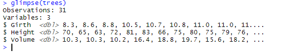
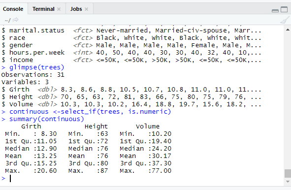
glimpse(trees)
To see categorical values factors are assigned.
levels(factor(trees$Girth))
// Verifying continuous variables
library(dplyr)

continuous <-select_if(trees, is.numeric)

summary(continuous)
// Including tree dataset in R search Pathattach(trees)
x<-glm(Volume~Height+Girth)

x
Output:
| Call: glm(formula = Volume ~ Height + Girth)
Coefficients: (Intercept) Height Girth -57.9877 0.3393 4.7082 Degrees of Freedom: 30 Total (i.e. Null); 28 Residual Null Deviance: 8106 Residual Deviance: 421.9 AIC: 176.9 |
summary(x)
| Call:
glm(formula = Volume ~ Height + Girth) Deviance Residuals: Min 1Q Median 3Q Max -6.4065 -2.6493 -0.2876 2.2003 8.4847 Coefficients: Estimate Std. Error t value Pr(>|t|) (Intercept) -57.9877 8.6382 -6.713 2.75e-07 *** Height 0.3393 0.1302 2.607 0.0145 * Girth 4.7082 0.2643 17.816 < 2e-16 *** — Signif. codes: 0 ‘***’ 0.001 ‘**’ 0.01 ‘*’ 0.05 ‘.’ 0.1 ‘ ’ 1 (Dispersion parameter for gaussian family taken to be 15.06862) Null deviance: 8106.08 on 30 degrees of freedom Residual deviance: 421.92 on 28 degrees of freedom AIC: 176.91 Number of Fisher Scoring iterations: 2 |
The output of the summary function gives out the calls, coefficients, and residuals. The above response figures out that both height and girth co-efficient are non-significant as their probability is less than 0.5. And there is two variant of deviance named null and residual. Finally, fisher scoring is an algorithm that solves maximum likelihood issues. With binomial, the response is a vector or matrix. cbind() is used to bind the column vectors in a matrix. And to get the detailed information of the fit summary is used.
To do the Like hood test, the following code is executed.
step(x, test="LRT")

Start:  AIC=176.91

Volume ~ Height + Girth

Df Deviance    AIC scaled dev.  Pr(>Chi)

<none>         421.9 176.91

- Height  1    524.3 181.65       6.735  0.009455 **

- Girth   1   5204.9 252.80      77.889 < 2.2e-16 ***

---

Signif. codes:  0 ‘***’ 0.001 ‘**’ 0.01 ‘*’ 0.05 ‘.’ 0.1 ‘ ’ 1

Call:  glm(formula = Volume ~ Height + Girth)

Coefficients:

(Intercept)       Height        Girth

-57.9877       0.3393       4.7082

Degrees of Freedom: 30 Total (i.e. Null);  28 Residual

Null Deviance:     8106

Residual Deviance: 421.9      AIC: 176.9
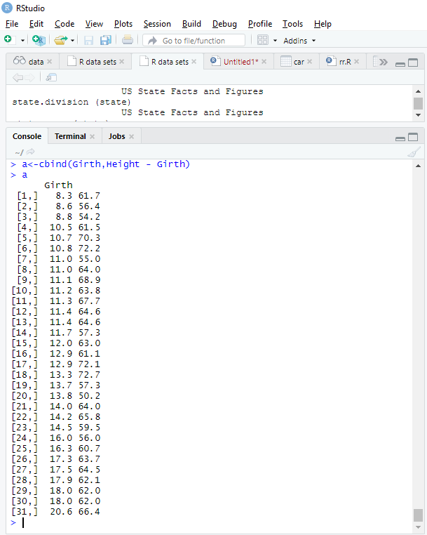
Model fit
a<-cbind(Height,Girth - Height)

> a
summary(trees)
Girth           Height       Volume

Min.   : 8.30   Min.   :63   Min.   :10.20

1st Qu.:11.05   1st Qu.:72   1st Qu.:19.40

Median :12.90   Median :76   Median :24.20

Mean   :13.25   Mean   :76   Mean   :30.17

3rd Qu.:15.25   3rd Qu.:80   3rd Qu.:37.30

Max.   :20.60   Max.   :87   Max.   :77.00
To get the appropriate standard deviation
apply(trees, sd)

Girth    Height    Volume

3.138139 6.371813 16.437846

predict <- predict(logit, data_test, type = 'response')
Next, we refer to the count response variable to modeled a good response fit. To calculate this, we will use the USAccDeath dataset.
Let us enter the following snippets in the R console and see how the year count and year square is performed on them.
data("USAccDeaths")

force(USAccDeaths)
// To analyze the year from 1973-1978.
disc <- data.frame(count=as.numeric(USAccDeaths),year=seq(0,(length(USAccDeaths)-1),1)))

yearSqr=disc$year^2

a1 <- glm(count~year+yearSqr,family="poisson",data=disc)

summary(a1)
| Call:
glm(formula = count ~ year + yearSqr, family = “poisson”, data = disc) Deviance Residuals: Min 1Q Median 3Q Max -22.4344 -6.4401 -0.0981 6.0508 21.4578 Coefficients: Estimate Std. Error z value Pr(>|z|) (Intercept) 9.187e+00 3.557e-03 2582.49 <2e-16 *** year -7.207e-03 2.354e-04 -30.62 <2e-16 *** yearSqr 8.841e-05 3.221e-06 27.45 <2e-16 *** — Signif. codes: 0 ‘***’ 0.001 ‘**’ 0.01 ‘*’ 0.05 ‘.’ 0.1 ‘ ’ 1 (Dispersion parameter for Poisson family taken to be 1) Null deviance: 7357.4 on 71 degrees of freedom Residual deviance: 6358.0 on 69 degrees of freedom AIC: 7149.8 Number of Fisher Scoring iterations: 4 |
To verify the best of fit of the model, the following command can be used to find
the residuals for the test. From the below result, the value is 0.
1 - pchisq(deviance(a1),df.residual(a1))
Using QuasiPoisson family for the greater variance in the given data
a2 <- glm(count~year+yearSqr,family="quasipoisson",data=disc)

summary(a2)
| Call:
glm(formula = count ~ year + yearSqr, family = “quasipoisson”, data = disc) Deviance Residuals: Min 1Q Median 3Q Max -22.4344 -6.4401 -0.0981 6.0508 21.4578 Coefficients: Estimate Std. Error t value Pr(>|t|) (Intercept) 9.187e+00 3.417e-02 268.822 < 2e-16 *** year -7.207e-03 2.261e-03 -3.188 0.00216 ** yearSqr 8.841e-05 3.095e-05 2.857 0.00565 ** — (Dispersion parameter for quasipoisson family taken to be 92.28857) Null deviance: 7357.4 on 71 degrees of freedom Residual deviance: 6358.0 on 69 degrees of freedom AIC: NA Number of Fisher Scoring iterations: 4 |
Comparing Poisson with binomial AIC value differs significantly. They can be analyzed by precision and recall ratio. The next step is to verify residual’s variance is proportional to the mean. Then we can plot using the ROCR library to improve the model.
Conclusion
Therefore, we have focussed on a special model called the generalized linear model, which helps in focussing and estimating the model parameters. It is primarily the potential for a continuous response variable. And we have seen how glm fits an R built-in packages. They are the most popular approaches for measuring count data and a robust tool for classification techniques utilized by a data scientist. R language, of course, helps in doing complicated mathematical functions.
Recommended Articles
This is a guide to GLM in R. Here, we discuss the GLM Function and How to Create GLM in R with tree data sets examples and output in a concise way. You may also look at the following article to learn more –
