FALSE Function in Excel (Table of Contents)
Introduction to FALSE Function in Excel
The FALSE function in Microsoft Excel is widely used. It is categorized under logical function/logical expression. The reason because it provides logical output. The one is the same as YES, NO, or 1, 0. It is a logical value for all such scenarios where the absence of anything or the non-possibility of any event occurs. FALSE is a compatibility function in Excel; therefore, it does not need to be called explicitly. It represents the Boolean value 0 (As in Boolean logic, TRUE =1 and FALSE = 0). This function can be widely used within conditional statements like IF, IFERROR, etc.
The syntax for the FALSE function is as below:
- This function does not have an argument and provides a logical FALSE value in a given Excel sheet. It is added under Excel primarily for maintaining compatibility with other worksheets as well as spreadsheet programs. This is similar to writing FALSE in any cell of your Excel worksheet. This means you do not even need to call this function. It can just be typed.
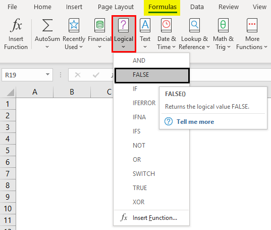
You can also find this function under the Logical category inside the Functional Library present in the Formulas tab in the Excel ribbon.
Examples of FALSE Function
Let’s take some examples to get going with the Excel FALSE function.
Example #1 – Using Logical Function’s Library
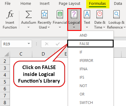
Step 1: Inside the given Excel sheet, click on the “Formulas” tab, and you will see a list of different Functional Libraries. Out of those, navigate to Logical and click on the drop-down arrow. A list of logical functions will appear. From there, select “FALSE” or click on “FALSE”.
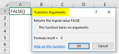
Step 2: As soon as you select and click on the FALSE function in your active cell formula FALSE will appear automatically, and with that, there will be a “Functional Arguments” window popping up, which consists of all the info associated with the FALSE function. Click OK in that pop-up window. It will return the logical FALSE as output in your working cell.
Step 3: You can directly type FALSE in your active sheet or =FALSE() to get the logical FALSE value. See the screenshot below.
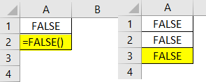
All these three methods are equivalent to each other for getting a logical FALSE value.
Example #2 – Using Logical Conditions in FALSE Function
We can use the FALSE function as an output to the logical conditions. Ex. Whether or not the given number is less than or greater than a particular number. We will see it step by step in the example below:
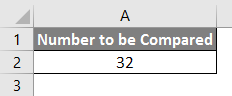
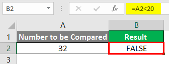
Step 1: Type any number in cell A2 of your working sheet. I will choose the number 32 and type it under cell A2.
Step 2: In cell B2, put a logical condition that checks whether 32 is less than 20 or not. You can type the following code under D2. =A2 < 20
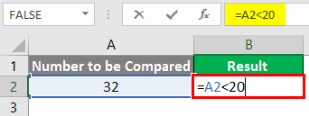
Step 3: Press Enter key to see the output of this formula. As we can see, the value present in cell A2 (i.e. 32) is not less than 20; therefore, the system will return logical FALSE as an output.
Similarly, you can get the output as FALSE when you check whether a value in cell A2 is greater than 50. I will leave it up to you to give it a try for this.
Example #3 – Using Mathematical Operations in FALSE Function
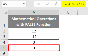
A FALSE function is a logical function equivalent to its Boolean value numeric zero (0). Therefore, all mathematical operations are possible with the FALSE function like we do those with numeric zero (0).
Step 1: Type the formula below in cell A2 of your active Excel sheet and press the Enter Key.
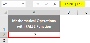
=FALSE() + 12
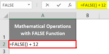
You get answer equivalent to (0 + 12).
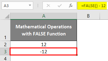
Step 2: In cell A3 of the active Excel sheet, type the following formula and press Enter.
=FALSE() – 12
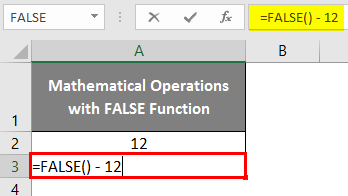
You’ll get output equivalent to (0 – 12).
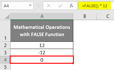
Step 3: In cell A4 of the active Excel worksheet, put the following formula and press the Enter key.
=FALSE() * 12
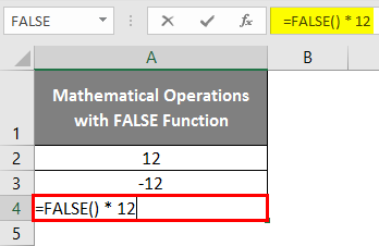
Since FALSE is equivalent to numeric zero, any number multiplied to it will be returning zero.
Step 4: In cell A5 of your active Excel sheet, use the formula below and press the Enter key.
=FALSE() / 12
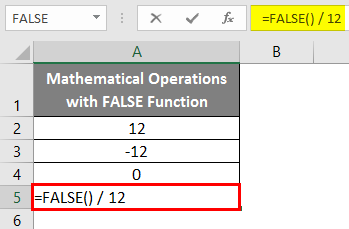
Again the same logic. As FALSE is equivalent to a numeric zero, the division of FALSE and any number would return a value of zero.
Example #4 – Using FALSE Function Under Logical Statements or Conditions
We frequently use the FALSE function under logical statements or conditions such as IF under Excel.
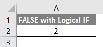
Step 1: In cell A2 of the active Excel sheet, put the number we want to check under the logical IF condition.
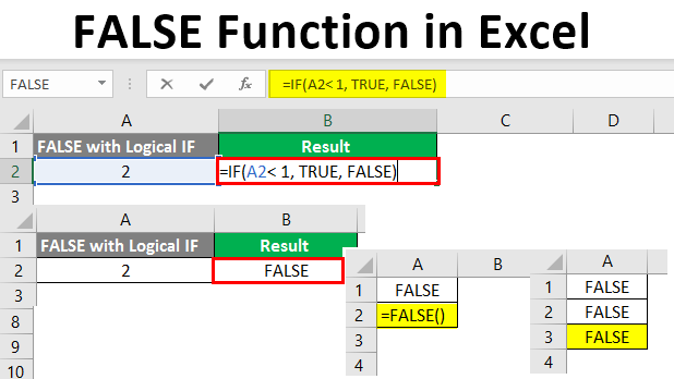
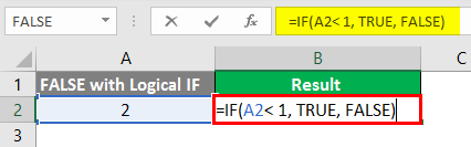
Step 2: Use the logical IF condition to check whether this number is less than 1. If it is less than 1, the output should be TRUE. Else, the output should be FALSE. Use the following conditional formula under cell C2 of the active worksheet. =IF(A2 < 1, TRUE, FALSE)
Press Enter key to see the output.
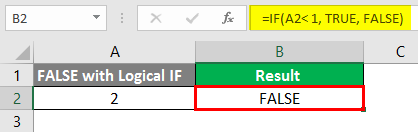
Since the condition A2 < 1 does not meet in this example, the system will generate an output as FALSE, equivalent to the FALSE function in Excel. Now, suppose we wanted the result as FALSE when A2 > 1; then, we can do it directly in the IF condition without using the else part with the help of the FALSE function.
In cell B3 of the active Excel sheet, put the following formula. =IF(A2 > 1, FALSE())
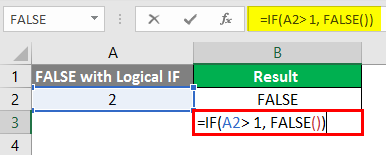
Press the Enter key.
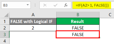
Here we have checked that if the value under cell A2 is greater than 1, it will give the output as FALSE directly. This example emphasizes that we can use the FALSE function within conditional outputs.
This is from this article. Let’s wrap things up with some points to be remembered.
Things to Remember About FALSE Function in Excel
- FALSE is equivalent to a numeric zero.
- The FALSE function does not require any argument to be called under Excel.
- This function does not even need parentheses to be added under it. This means FALSE and FALSE() are identical.
Recommended Articles
This is a guide to FALSE Function in Excel. Here we discuss How to use the FALSE Function in Excel, practical examples, and a downloadable Excel template. You can also go through our other suggested articles –
