Table of Contents
Spreadsheet Formulas in Excel
A spreadsheet is full of formulas. Firstly don’t get confused with the spreadsheet and worksheet; both are the same. This article will talk about the most important formulas in excel and how do we use them in our day-to-day activities.
How to Use Spreadsheet Formulas in Excel?
Spreadsheet Formulas in Excel are very simple and easy to use. This is the guide to Formulas in Excel with Detailed Spreadsheet Formulas Examples. Let’s understand how to use Spreadsheet Formulas in Excel with some examples.
Example #1
SUMPRODUCT Formula in Excel Spreadsheet
If we want to do unit price * unit sold calculation, we will do an individual calculation and finally add the total to get the total sales. For example, look at the below example.
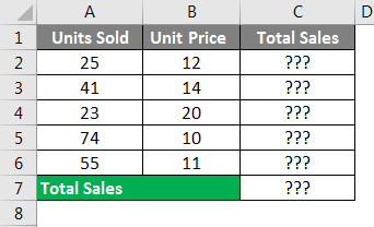
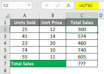
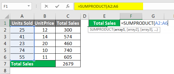
Firstly we calculate the total sales by multiplying Units Sold to Unit Price, as I have shown in the below image.
Finally, we add the total of sales to get the final total sales amount.
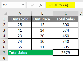
This includes many steps to get the final sales amount. However, using the SUMPRODUCT function, we can get the total in a single formula itself.
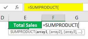
In the first array, select Units Sold range.
We need to do the multiplication, so enter an asterisk (*) symbol and select Unit Price.
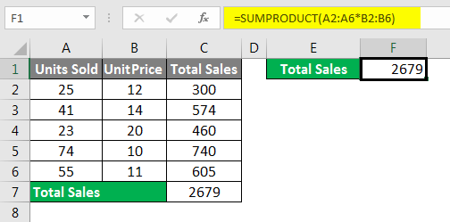
Oh yes, we got our end result in a single formula in a single cell itself. How cool is it?
Example #2
Formula to SUM Top N Values in Excel Spreadsheet
We all work on the SUM function in Excel Spreadsheet in Excel day in day out in an Excel Spreadsheet; this is not a strange thing for us. But how do we sum the top 3 values or top 5 values, or top X values?
It looks like a new thing isn’t it? Yes, we can SUM Top N values from the list. For example, look at the below data.
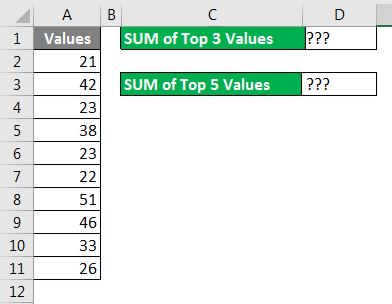
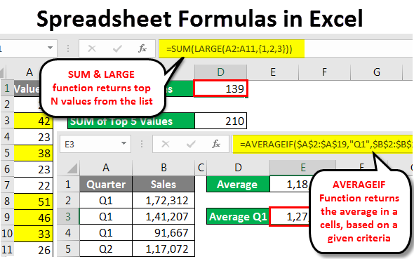
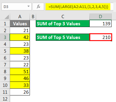
With the combination of SUM & LARGE function in an Excel Spreadsheet, we can sum the top n values from the list. The LARGE function helps us to find the top largest value.

In order to find the top 3 values, I applied the SUM function formula for this SUM function. I have entered one more function, LARGE, to get the top N values. A LARGE function in Excel Spreadsheet can return only one largest in order to find the top N values. We need to supply the numbers in curly brackets ({). Now LARGE will return the top 3 largest values, and the SUM function will add these 3 numbers and give us the total.
Similarly, if I want the sum of the top 5 values from the list in the Excel Spreadsheet, I need to supply the numbers to 5 in curly brackets. Now LARGE will return the top 5 largest values, and the SUM function will add these 5 numbers and give the total.
Example #3
SUMIF Formula with Operator Symbols in Excel Spreadsheet
You must have worked with the SUMIF function while using Excel Spreadsheet, and you are perfectly alright as well. But we can pass the criteria to the SUMIF function formula with operator symbol as well. For an example, look at the below example.
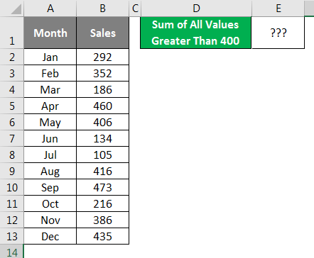
We need to do the addition of all the values which are greater than 400. For sure, we need to use the SUMIF function, but in criteria, we need to supply an operator symbol greater than (>) and mention the criteria as 400.
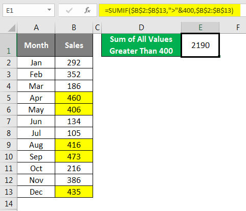
Yes, we need to supply the criteria operator symbol in double quotes (” “) and combine the other criteria with the ampersand (&) symbol. Now formula will read it as greater than 400 and returns the total.
I have marked all the values which are greater than 400 with yellow color; you can add those values manually you will get the same total as 2190.
Example #4
Table for All kind of Calculations in Excel Spreadsheet
Often we need to do the summation of values; often, we need the count, often the Average of the numbers, and many other things. How do you deal with all these requirements in a single formula?
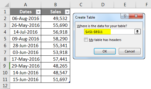
Assume below is the data you have in your Excel Spreadsheet.
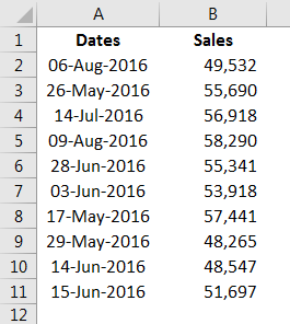
Step 1: Convert this range to the table by pressing Ctrl + T.
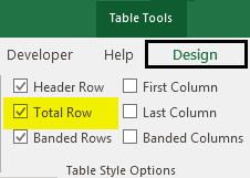
Step 2: Place a cursor inside the table > go to Design > Under Table Style Options check the option Total Row.
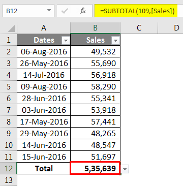
Step 3: Now, we have a total of the table row at the end of the table.
Step 4: But if you observe, it is not the only formula; rather, it has a drop-down list. Click on the drop-down list to see what more has in it.
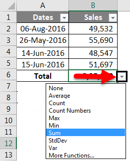
Using this drop-down, we can use Average, Count, find the Max value, find the Min value, and many other things as well. Based on the selection we make from the drop-down, it will show the results.
Example #5
AVERAGEIF Formula in Excel Spreadsheet
AVERAGE function is not a strange thing for us. At the point of time, if we need the average of values, we would apply the AVERAGE function formula in Excel Spreadsheet and get the result. For example, if I need the average of the below numbers, I would apply the AVERAGE function.
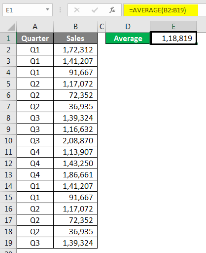
What if we need an Average only for the quarter Q1? How do we do? We can do with manual work, but we all hate manual work isn’t it?
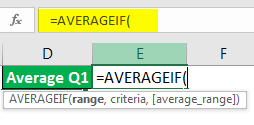
Nothing to worry about; we have a function called AVERAGEIF in Excel Spreadsheet.
The range is nothing but our Quarter Range, so select Quarter range from A2 to A19.
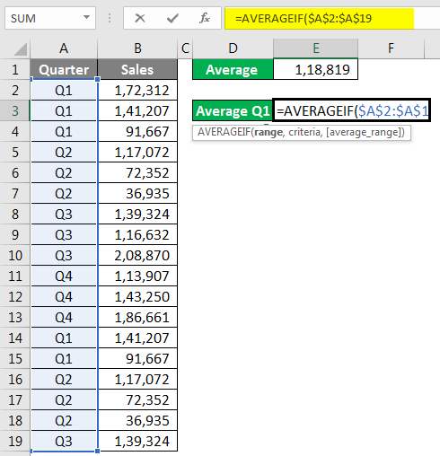
Criteria are what you want to do from this range. Our criteria are Q1.

The average Range is nothing but the sales column to select the Sales column and close the bracket. We will get Q1 Average Only.

Example #6
IFERROR Formula to Avoid Errors in Excel Spreadsheet
I am sure you have encountered many errors while applying formulas. Often, we need to ignore these errors and clear these error values as per our own values, especially when creating and managing reports. For example, look at the below illustrations.
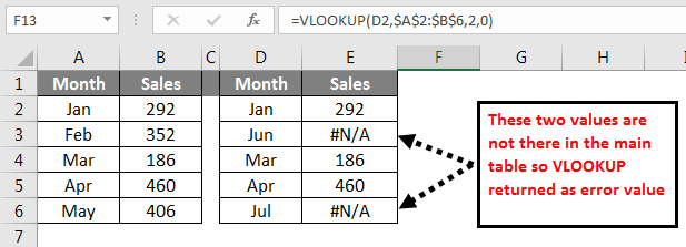
In the above image, we got error values. I want to convert all the error values to Not Found. Apply the below formula to get the result.
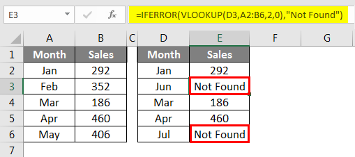
If VLOOKUP returns an error values IFERROR convert this to Not Found text value.
Example #7
TEXT Function to Concatenate Date Values in Excel Spreadsheet
Using CONCATENATE function, we can combine many cell data into one. But this does not work a similar way if you are combining dates with text in Excel Spreadsheet. Look at the below image.
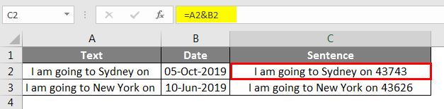
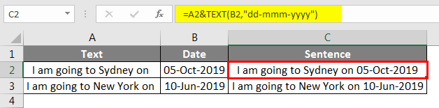
When I combined cells A1 & A2, I got the result of these two cell values. However, a date is not in the correct format; in order to make this a perfect format, we need to use the TEXT function to apply our date format.
Below is the formula which can make this a proper sentence.
Example #8
TEXT Function to Concatenate Time Values in Excel Spreadsheet
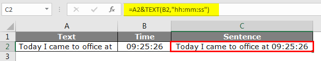
Like how we got an incorrect format for date similarly for time format, also we get incorrect format.

We need to pass the time cell with the TEXT function and convert it to “hh:mm:ss” format in Excel Spreadsheet.
Things to Remember
- Using CONCATENATE function, we can combine many cell data into one.
- In order to make the Date Format correct, we need to use the TEXT function to apply our date format.
- By using the SUMPRODUCT function, we can get the total in the single formula itself.
Recommended Articles
This has been a guide to Spreadsheet Formulas in Excel. Here we discussed different Spreadsheet formulas in Excel, How to use Spreadsheet Formulas in Excel, along with practical examples and downloadable excel template. You can also go through our other suggested articles-