Excel Data Bars

What are Data Bars in Excel?

Data bars in Excel is an option that you can use to create bar graphs inside the cells. It is an inbuilt conditional formatting option that lets you compare different values by only looking at the length of the data bar.

Generally, if the data bar is longer, it means that the value is larger than others and vice versa. These bars are also color-coded, making it easy to quickly find trends and differences in your data without analyzing the data.

For instance, consider you have a list of temperatures ranging from 15°C to 40°C. If you add colored data bars for each temperature, the 15°C will display a short blue bar, and the 40°C may display a long red bar (color depends on the pattern you choose).

Table of Contents

• What are Data Bars in Excel?
• How to Add a Data Bar?
• Examples
  • Custom Solid Color Data Bars
  • Custom Gradient Color Data Bars
  • Positive and Negative Data Bars
  • Without Numbers Data Bars
• Advanced Features

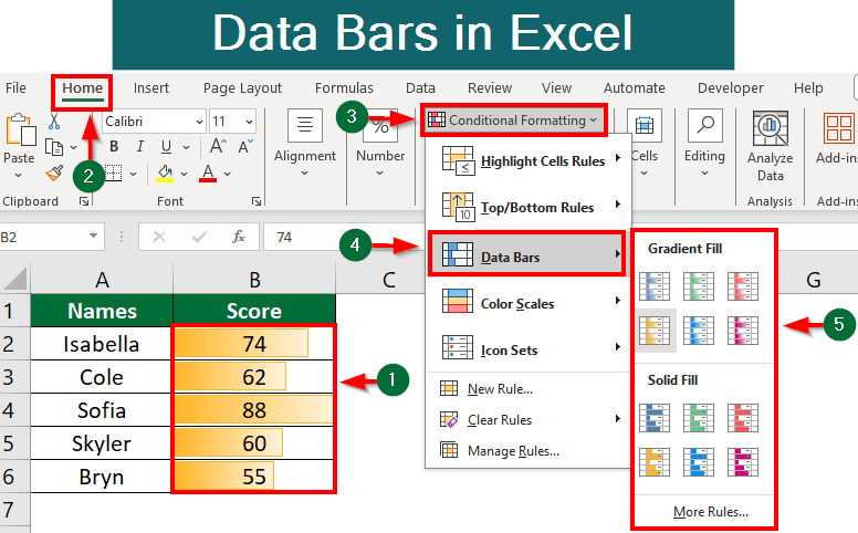
How to Add Data Bars in Excel?

1. Select the data range.
2. Go to the Home tab.
3. Click the Conditional Formatting dropdown button in the Styles group.
4. Choose Data Bars. You will have two options: Gradient Fill or Solid Fill. Select your choice.

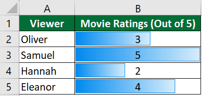
For example, we have a table of movie ratings, for which we have added data bars following the steps shown below.

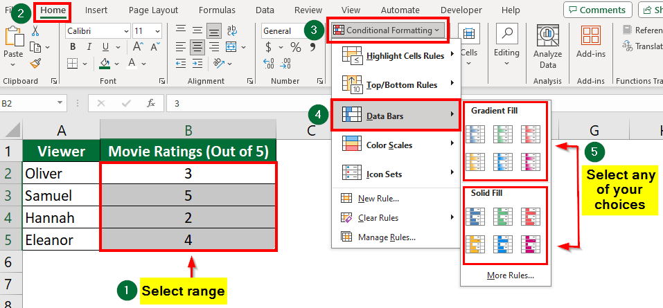
Result: We have added gradient color data bars.

Examples of Data Bars in Excel

Here are a few examples of how to use data bars in Excel in different ways.

#1. Custom Solid Color Data Bars

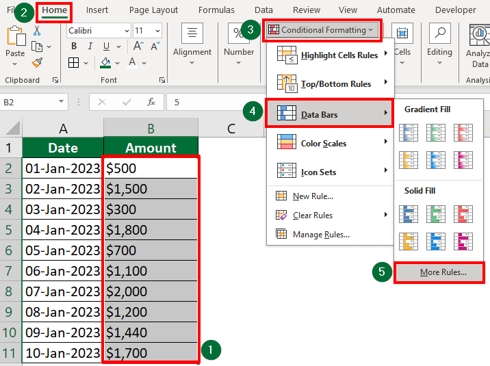
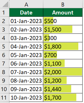
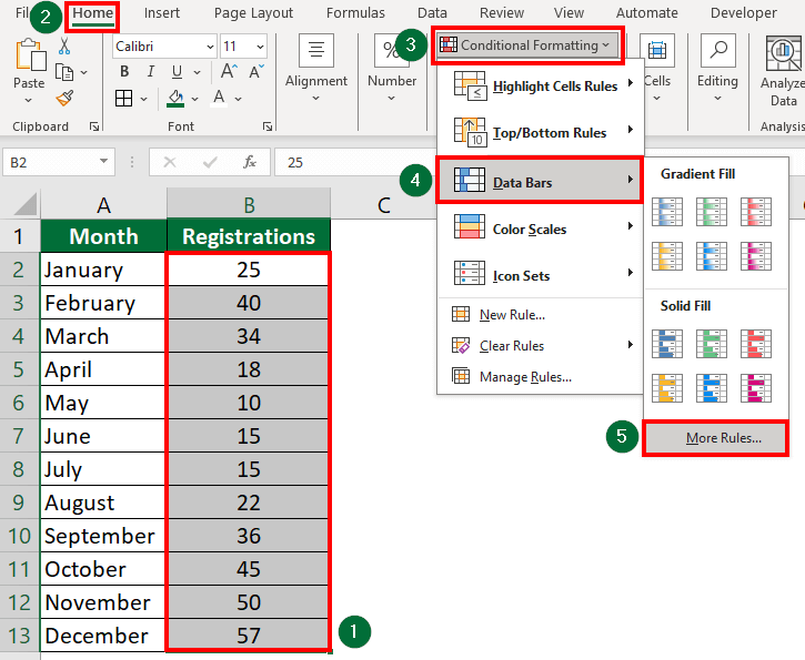
Suppose Daniel has a table that records his daily expenditures. He wants to highlight the amount he spends each day by applying data bars in Excel.

Let’s find out how he can do that:
1. Select the range B2:B11
2. Go to the Home tab on the Excel ribbon.
3. Open the dropdown menu for Conditional Formatting.
4. Choose Data Bars.
5. Select More Rules from the bottom of the Data Bars submenu.

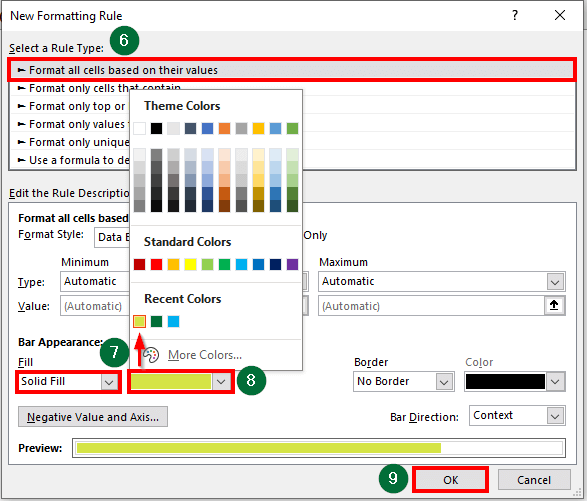
6. A dialogue box will appear where he must choose “Format all cells based on their values”.
7. Then, in the Bar Appearance, choose Solid Fill.
8. Next, he selects the color of his choice.
9. Click OK.

Result:
Using the data bars, we can see that Daniel spent the lowest on 3rd Jan ($300) and highest on 7th Jan ($2,000).

#2. Custom Gradient Color Data Bars

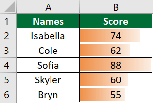
Abigail is a teacher who wants to find which students got the highest score in her class using data bars in Excel.

Here are the steps that Abigail will follow:
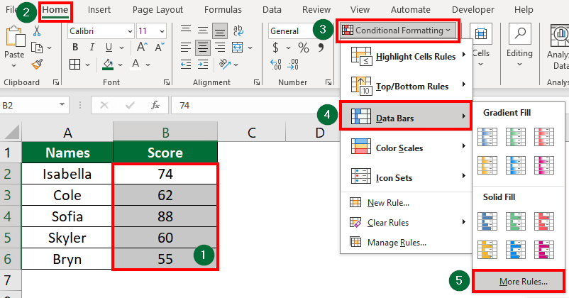
1. Selecting the range, for instance, B2:B6
2. Opening the Home tab.
3. Selecting the Conditional Formatting option.
4. Clicking on Data Bars.
5. Selecting More Rules.

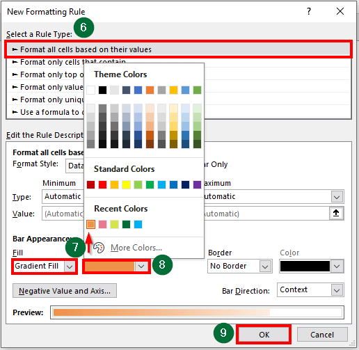
6. In the dialogue box, she will choose “Format all cells based on their values”.
7. Next, in Bar Appearance, she selects Gradient Fill.
8. Then, she selects orange as her color of choice.
9. Finally, she clicks on OK.

Result:
Abigail finds that, as per the data bars, Sofia is the topper with an 88 score.

#3. Positive and Negative Data Bars

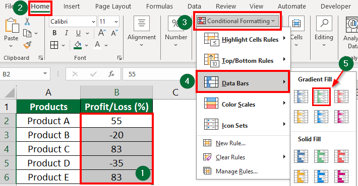
Bryan, a Sales Manager, wants to see which of his products generate profits and which are incurring losses. Thus, he uses data bars in Excel to perform this task.

Steps that Brian performs:
1. He selects the range with the data (B2:B6).
2. He opens the Home tab.
3. Then, he opens the dropdown menu for Conditional Formatting.
4. After that, he chooses Data Bars from the dropdown.
5. Next, he selects the Gradient Fill Option.

Result:
Excel automatically applies gradient color data bars to the selected cells. It displays the positive values in green and the negative values in red. Through this, Bryan discovers that Products A, C, and E are making profits, and Products B and D are making losses.

#4. Without Value Data Bars

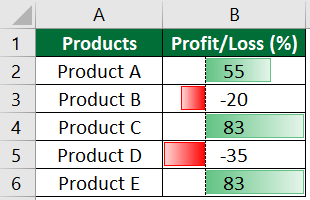
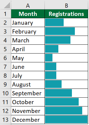
Vtravellers, a tourism company, wants to see how many people registered for their services each month of the year, but they don’t want to see the actual numbers. Instead, they want a visual representation using bars.

To do so, they use data bars in Excel in the following way:
1. Choose the range, i.e., B2:B13
2. Go to the Home tab on the Excel ribbon.
3. In the Styles group, open the Conditional Formatting dropdown.
4. Choose Data Bars from the list.
5. Click on More Rules.

 

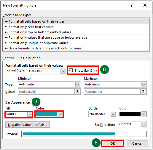
6. In the New Formatting Rule dialog box that appears, check the “Show Bar Only” Option.
7. Customize the Bar Appearance as per your choice.
8. Click on the OK button.

Result:
We can see that Vtravellers received the highest number of registrations in the month of December.

Advanced Features

1. Axis Position

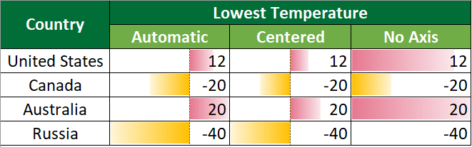
When making data bars, you can choose their alignment in the cell using the Axis setting. You have three options:

1. Automatic: Excel sets the data bars based on your data. If you have both positive and negative numbers, the center of the data bar will be present where the value 0 is, then the right will be for positives, and the left will be for negatives.
2. Centered: The data bars’ axis is always in the center of the cell. Positives extend right, and negatives extend left.
3. No Axis: Data bars fill the entire cell from left to right, regardless of your data. There is no reference axis.

These axis positions look like this:

To apply data bars with a specific axis position in Excel, follow these steps:

1. Select the range of cells.
2. Go to the Home > Conditional Formatting > Data Bars and click More Rules.
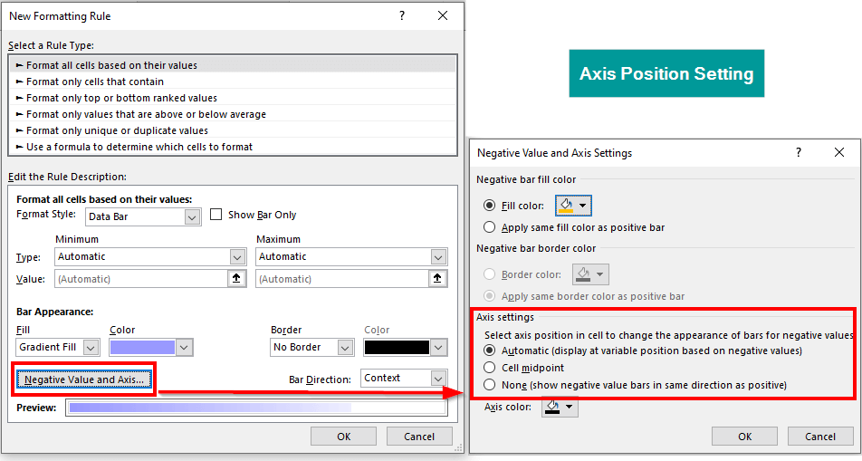
3. Click on Negative Value and Axis.
4. In the submenu that appears, you will see options for “Automatic,” “Cell Midpoint,” and “None.” Select your desired axis position.
5. Click OK and again OK.

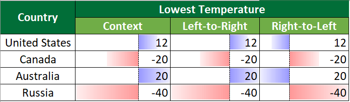
2. Data Bar Direction

You can customize the direction of data bars. You can choose whether they fill from left to right or right to left.

Here are the three data bar direction options:

1. Context (default): Excel automatically sets the direction based on values. Positive values fill left-to-right, and negative values fill right-to-left.
2. Left-to-Right: It is similar to the context (default) direction. Here, the data bars always fill left to right.
3. Right-to-Left: Data bars always fill right-to-left, meaning that the highest negative value is at the right, and the positive values are on the left.

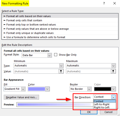
To set the direction of data bars in Excel:

1. Select the cells > Go to the Home tab > Conditional Formatting > Data Bars > Select More Rules.
2. In the dialog box that opens, click on Bar direction.
3. From the dropdown, select any of the three options and click OK.

3. Minimum and Maximum Data Bars

Excel sets default minimum and maximum values for data bars. Usually, the minimum/maximum value is the highest number in the dataset (it can be negative or positive). But you can also customize them using a custom rule.

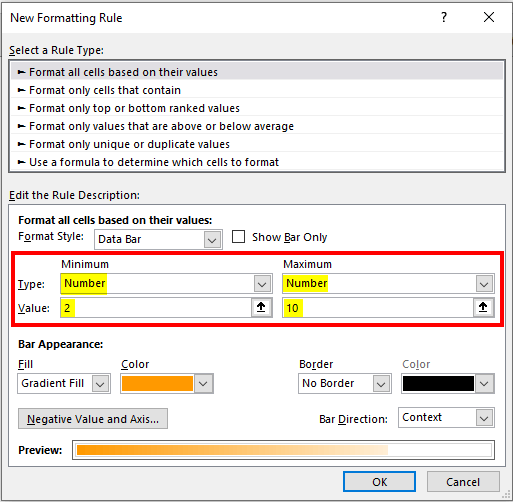
Here’s how to customize the minimum and maximum data bar values:

1. Select the data range > open the Home tab > Click on Conditional Formatting > hover your mouse over Data Bars > More Rules.
2. The New Formatting Rule dialog box will appear. You can see the Minimum and Maximum
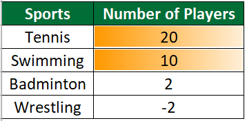
3. In the Minimum box, select Type as Number and Value as “2”.
4. In the Maximum box, choose Type as Number and Value as “10”.
5. Click OK.

Result:
The cell with the maximum value will have a bar filling the entire cell, while there will be no data bar for the value that you set as a minimum.

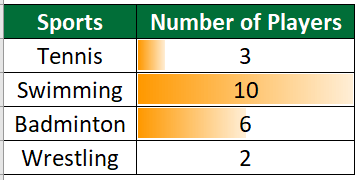
Note:

1. Any value that is lower than the minimum value will not have a data bar. For instance, in the image below, -2 does not have a data bar because it’s less than the minimum value (2).
2. If a value is higher than the maximum value, it will get the same data bar length as the maximum value. For instance, in the image below, the value 20 has the same data bar length as the maximum value (10).

Frequently Asked Questions(FAQs)

Q1. How can I add data bars to a Pivot Table in Excel?
Answer: You can add data bars to a pivot table in Excel by selecting the cells within the pivot table and then applying the conditional formatting as you would do for any other range of cells.

Q2. Can I use data bars with other types of conditional formatting?
Answer: Yes, you can combine data bars with other types of conditional formatting in Excel to create more complex formatting rules. When you manage your rules, you can also adjust the order in which they are applied.

Q3. Can I copy and paste cells with data bars to other worksheets or workbooks?
Answer: Yes, you can copy and paste cells with data bars to other worksheets or workbooks, and the formatting should remain intact as long as the target workbook supports data bars.

Recommended Articles

This article is a guide to Data Bars in Excel. Here, we discuss how to add data bars in Excel with Excel examples and a downloadable Excel template. You may also look at these useful charts in Excel –

1. Excel Bar Chart
2. Formula Bar in Excel
3. Stacked Area Chart
4. Status Bar in Excel