Updated August 23, 2023
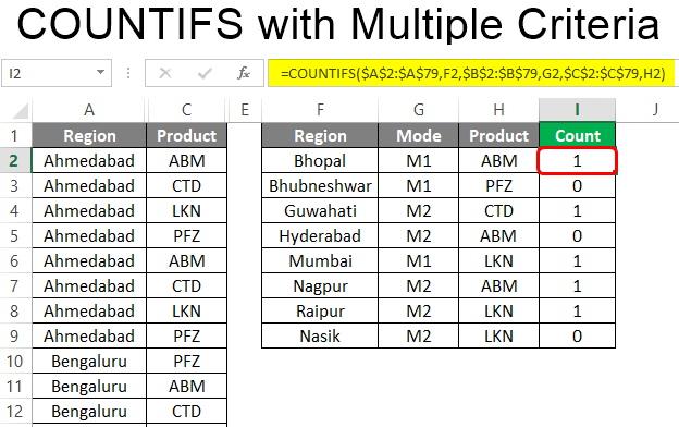
COUNTIFS with Multiple Criteria (Table of Contents)
Introduction to COUNTIFS with Multiple Criteria
Excel provides us COUNTIFS function to return a count if certain conditions are met. The function purely works for multiple conditions. This technique is quite useful in complex calculations that involve a huge dataset. COUNTIFS takes multiple parameters as input, but the parameters are of only two types: Condition value and range in which condition value will search.
How to Use COUNTIFS Function in Excel?
We will go through a step-by-step procedure to implement and use counties with multiple criteria in Excel. For this demonstration, we will use Volume distributed to various regions of India. Volume is a measure in the dataset, given by Region, Mode, and Product dimensions. Mode essentially refers to the distribution mode. We’ll use counties to return the count based on multiple criteria. Let’s go through the following section to understand this.
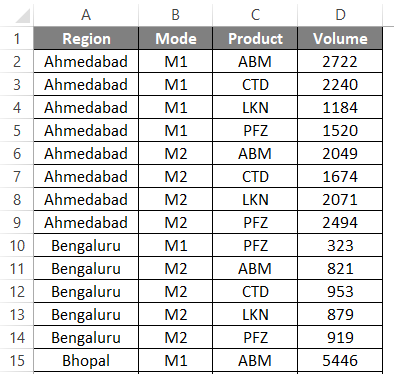
- First, have a look at the data, which is shown in the following screenshot. Observe the dimensions and the measure present in the dataset.
- As we can see, going through the dataset, we have three dimensions that form three criteria columns. We may want a count based on the criteria column above. Now, imagine we want to count for conditions as shown in the following table.
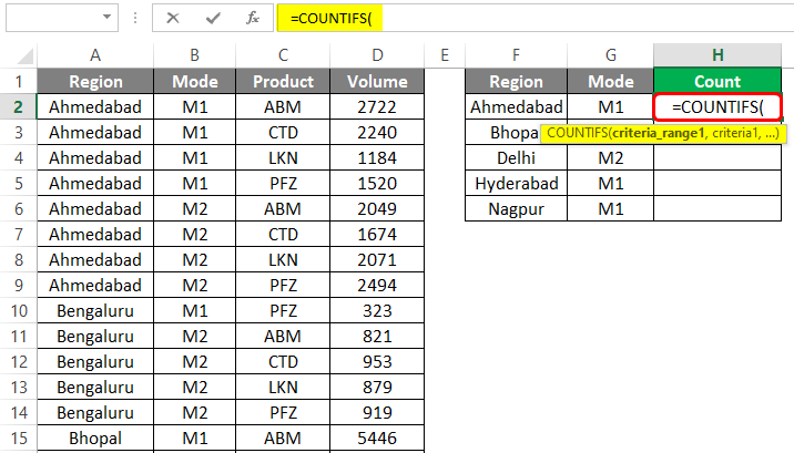
- As we can see above, we want to know the count based on the criteria represented by the two columns. Here, by criteria, to give an example, we essentially mean that count the number of entries for which Region is Ahmedabad, and Mode is M1. This task seems difficult, but Excel provides a very easy approach through the COUNTIFS function. Let’s first see how the COUNTIFS function works.
As seen in the above screenshot, Excel automatically shows what parameters need to be passed into the counties function when we enter the counties function. The COUNTIFS function takes multiple criteria ranges and corresponding criteria. The first criteria range and criteria appear as criteria range1 and criteria1.
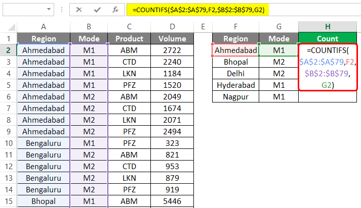
- We will use the COUNTIFS function now. For this, let’s pass the input parameters properly. The first parameter is the criterion range. Here, the criteria range is the range in the table in which we want to search for counting. In this case, the first criteria range would be the Range column, and the criterion would be the region name that needs to be searched in the range. The criterion must select from the table where we want the value. The following screenshot shows how the table passes the first criterion range and criterion as parameters.
Do not just forget to make the criteria range constant (append $ sign in the range), as seen in the above screenshot.
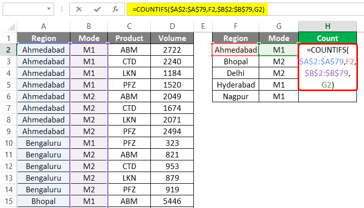
- We also have another criterion to be met. This is on mode. For this, follow the same procedure we followed for the first criterion except that we would select the Mode column and the criterion range2 from the dataset, and the corresponding value for mode in the other table as the criterion. The implementation is shown in the following screenshot.
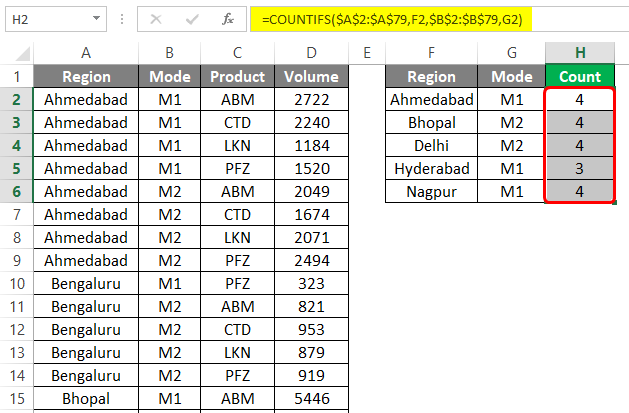
- Now, once done, close the function and press enter. Observe if we get the correct result. As shown in the screenshot below, the COUNTIFS function has returned the value 4, which shows that for region Ahmedabad, mode value M1 appears four times. This correctness can verify by reviewing the dataset. Let’s implement this function for other region values in the table. For this, copy the function for these entries. Doing this gives us the corresponding count values, as seen in the following table.
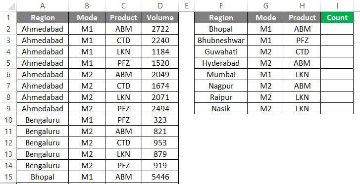
- So, the COUNTIFSS function makes the seemingly difficult task very easy. The above example we saw had two criteria. Now, we also have a third dimension in the table: the Product. Let’s imagine we want to identify the number of entries with a particular region that used one of the two modes for a certain product. So, this necessarily means that we have three criteria. Well, the implementation of COUNTIFS won’t differ much from what we saw previously. We shall now have a third criteria range and corresponding criteria related to the Product dimension. The table containing the criteria is shown below. We want to return the count based on these criteria.
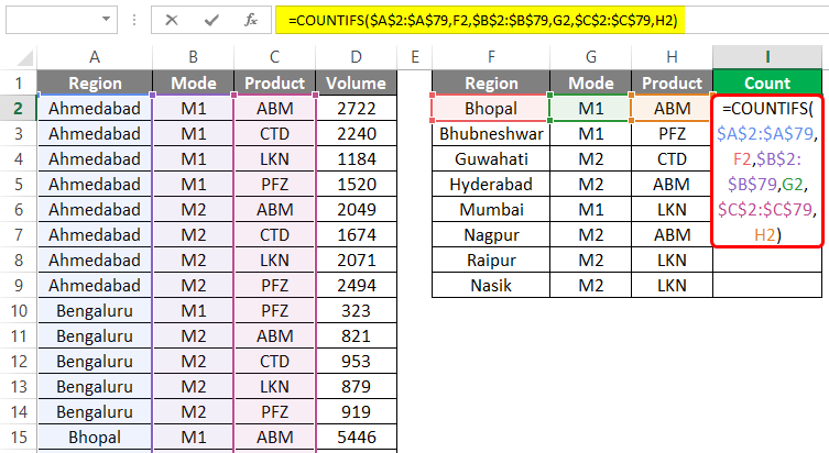
- The following screenshot shows the COUNTIFS function’s implementation to return count based on three conditions, as shown in the above table. Observing the screenshot, we can say that it is just an extended version of the COUNTIFS implementation that we saw previously.
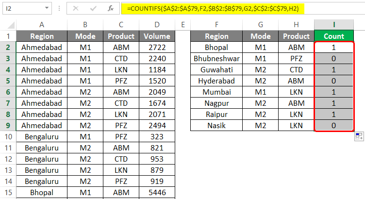
- Upon implementing the function, we obtain the value 1, indicating that one entry satisfies all three criteria. Let’s copy the function across all the desired cells. Doing this, we get the result shown in the following table.
As we can see above, for certain entries, we have got zero. This means that there exist no such entries in the dataset. We got the value 1 for the remaining entries, meaning that such combinations are present.
Things to Remember about COUNTIFS with Multiple Criteria
- The COUNTIFS function in Excel must be used only when there are two or more criteria. For dealing with a single condition, Excel provides other mechanisms.
- While implementing the COUNTIFS function, selecting the criterion range and criterion from the correct sources is crucial, as otherwise, the result would be incorrect.
Recommended Articles
This has been a guide to COUNTIFS with Multiple Criteria. Here we discuss How to use COUNTIFS with Multiple Criteria, practical examples, and a downloadable Excel template. You can also go through our other suggested articles –
