Updated August 19, 2023

Conditional Formatting Based on Another Cell
Conditional Formatting can be a lifesaver when you have a spreadsheet full of data and want to highlight only the necessary information. However, conditional formatting is not just limited to highlighting specific cells. It also helps format a cell based on the value of another cell. This type of formatting is known as conditional formatting based on another cell value.
Let’s say you’re a teacher and keep track of your student’s grades using Excel. You can use conditional formatting based on another cell to highlight grades equal to or greater than 90. This way, you can quickly identify students excelling in your class. You can even highlight those grades in green, making them easier to identify.
In this article, we will understand the basics of conditional formatting based on another cell and provide examples of how it can enhance the presentation and analysis of spreadsheet data. Before moving to the complex examples, let’s first understand the location of the conditional formatting option in Excel.
Where is Conditional Formatting in Excel?
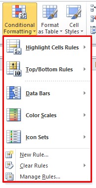
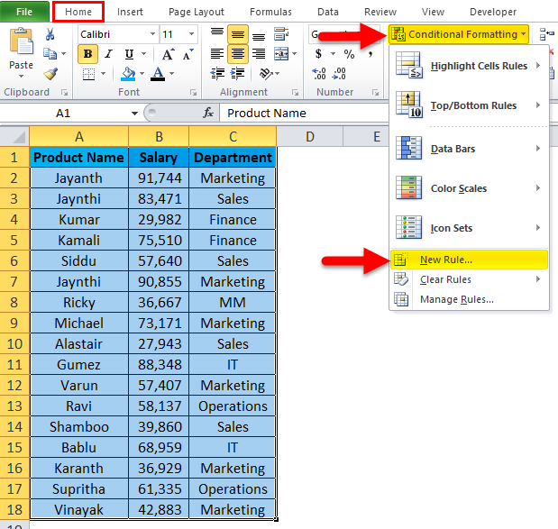
The Conditional Formatting option is under the Home tab in the Styles group section. By clicking on conditional formatting, you will find many options like Highlight Cells Rules, Data Bars, Manage rules, etc.
How to Apply Excel Conditional Formatting Based On Another Cell Value?
Example #1
Method 1: Highlight Single Cell Value
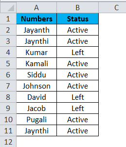
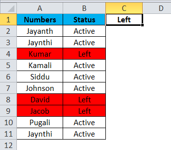
Below is simple data on employees’ current status as “Active” and “Left”. Here, “Active” means employees still in service, whereas “Left” denotes employees who have left the organization.
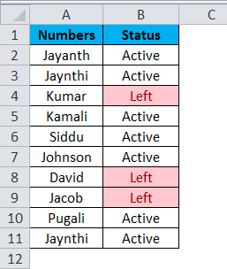
In this method, you will learn how to highlight all the employees with the status “Left” in the below data using the single-cell value formatting technique. It will highlight only the individual cell which contains the text “Left”.
Please follow the below steps to learn this technique.
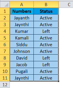
Step 1: Select the entire data.
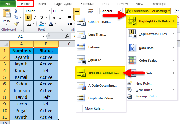
Step 2: Go Home, select Conditional Formatting > Highlight Cells Rules > Text That Contains.
Step 3: When you click on the Text that contains, a new window will open as shown below. Enter the text value you want to highlight, i.e., Left, and then select the color format as Light Red Fill with Dark Red Text. Click on the OK option to complete this task.
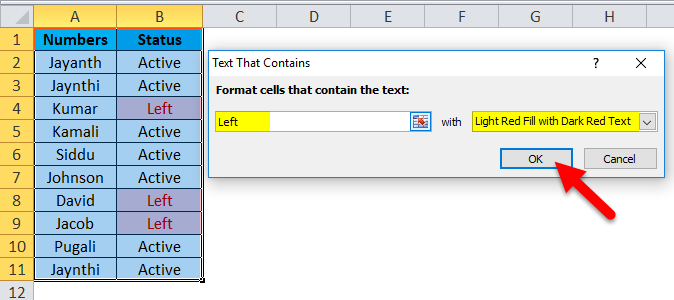
You can also see the preview of this task in the data. The output is displayed below:
Method 2: Highlight the Entire Row Based on One Single Cell Value
In the previous example, we have seen how to highlight a single cell based on the cell value. In this example, you will learn how to highlight an entire column based on the single-cell value. Please follow the below steps to accomplish this task.
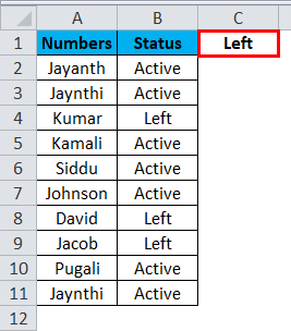
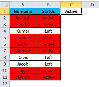
Step 1: Enter the “Left” word in cell C1.
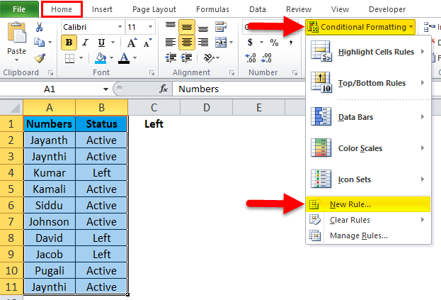
Step 2: Select the entire data. Now, go to Home, click Conditional Formatting > New Rule.
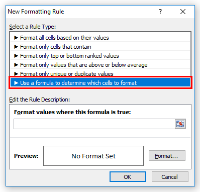
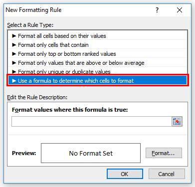
Step 3: The New Formatting Rule window will open; select Use a formula to determine which cells to format.
Step 4: In the formula section, enter the formula =$B2=$C$1 (as shown in the image below) and click Format.
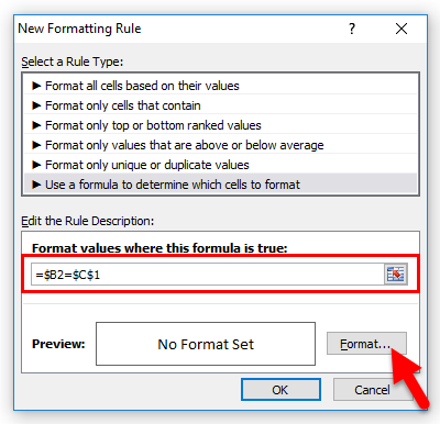
The formula states that If the B2 cell is (this is not an absolute reference, but the only column is locked) equal to the value in the C1 cell (this is an absolute reference), then do the formatting.
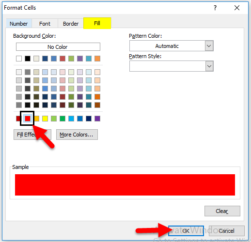
Step 5: In the Format Cells window, click the Fill option, select the formatting color, and click the OK button. The preview section will display the color you choose.
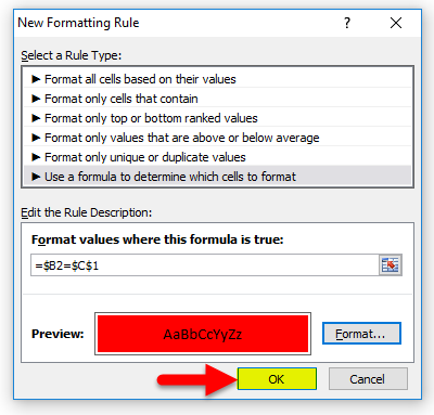
Step 6: After opening the New Formatting Rule window, click OK again to format the rows if the cell value equals the left text.
The outcome is as follows:
Now try changing the cell value in C1 from Left to Active. It will highlight all the Active row employees.
Example #2
We have an employee database with names, salaries, and departments. Here we want to highlight the departments of Marketing and IT. We must apply the formula in the conditional formatting tab to do this task.
Step 1: Select the entire data.

Step 2: Click on Conditional formatting > New Rule.

Step 3: Select Use a formula to determine which cells to format.
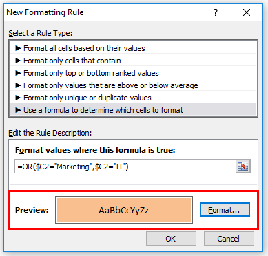
Step 4: In the formula section, enter the formula =OR($C2=”Marketing”,$C2=”IT”) and click on the Format button.
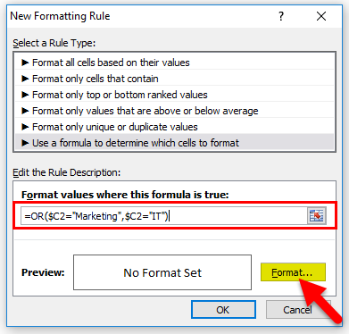
Step 5: Click on Format and select the color you want to highlight. The preview section will display the color.
Step 6: Click on OK to complete the task.
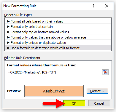
The Conditional Formatting formula has highlighted the departments of Marketing or IT.

Example #3
In this example, we want to highlight all the Marketing department rows with a salary of more than 50,000.
Step 1: Select the entire data.

Step 2: Click on Conditional formatting>New Rule.
Step 3: In the New Formatting Rule window, select Use a Formula to determine which cells to format.

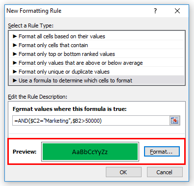
Step 4: Under the formula section, enter the formula =AND($C2=”Marketing”,$B2>50000) and click on Format.
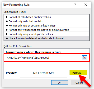
Step 5: Select the color you want to use for highlighting. We have selected the below color shown in the below image.
Step 6: Click on the OK button.
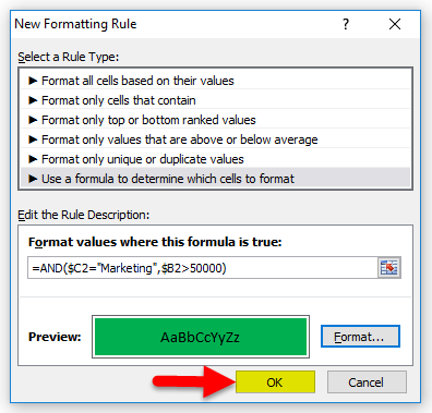
The above formula will highlight all the rows with Marketing and salary of more than 50,000.

In the above image, the marked yellow rows are also Marketing, but the salary is less than 50,000, so AND function excludes these rows from highlighting.
Things to Remember
- You can use conditional formatting to spot variances, specific words, or characters in cell values.
- You can also differentiate your data by changing the cell color, border styles, font color, etc.
- To create conditional formatting formulas and rules, you must understand the range and condition clauses.
- To format cells, you can use predefined features like data bars, color shades, and icons.
- You can delete/clear the highlights after applying the formatting rule.
- Suppose you plan to add additional data and want the conditional formatting rule to apply automatically to new data. In that case, you can convert that data into a table from the insert tab. All new rows will automatically receive conditional formatting rules.
Common Mistakes to Avoid
- You must know what condition rules will give the desired results, like greater than, less than, or equal to.
- You must know which is an absolute cell & relative cell to address them correctly.
- Avoid using the symbol “$” in unnecessary places. Please remember that =D1=1, =$D$1=1, and =D$1=1 will produce different results.
- Avoid including the column headers when selecting cells or data.
Best Practices for Sharing Spreadsheets with Conditional Formatting
- Check all the conditional formatting rules and formulas applied to the data before sharing the spreadsheet.
- If you do not want to share the spreadsheet with highlights, remove or delete the highlighted cells/rows using the “Clear rules” option. Click Home>Conditional formatting>Clear rules>Clear Rules from Selected cells
You can give members like edit/view(read-only) access to avoid unnecessary changes in the spreadsheet.
Frequently Asked Questions (FAQs)
Q1. What is conditional formatting in Excel?
Answer: Conditional formatting in Excel mainly highlights specific information or data in a worksheet. It changes the appearance of the cell for easy identification.
Q2. How to remove conditional formatting in Excel?
Answer: Firstly, select the data where conditional formatting rules are applied. To clear the
highlight, follow the below steps.
Select Conditional formatting>Clear rules>Clear Rules from Selected cells
Q3. How to copy conditional formatting in Excel?
Answer: Please follow the instructions to copy the conditional formatting rule using Format Painter.
- Select the cells that have the conditional formatting rule you want to copy.
- Go to Home> Clipboard>Format Painter.
- Select the cells to which you want the copied formatting to apply.
Recommended Articles
This article has been a guide to “Conditional Formatting Based On Another Cell”. Here we discuss applying conditional formatting in Excel based on single and other cell values with practical examples and downloadable Excel templates. You can also go through our other suggested articles –
