Excel Compare Two Columns (Table of Contents)
- How to Compare Two Columns in Excel Using VLOOKUP?
- Examples of Compare Two Columns in Excel using VLOOKUP
Compare Two Columns in Excel using VLOOKUP & Find Data
While working with data in Excel, sooner or later, you will need to compare two columns to check whether data from one column is present in another column or not. When it comes to making comparisons between two columns, lookup functions are the best in business. We can use the VLOOKUP function to compare whether two columns have matching data within them or not. This function saves you a lot of time while working on a large amount of data where you must compare two columns, increasing productivity and reducing the time a task takes to complete.
How to Compare Two Columns in Excel Using VLOOKUP?
When we have two columns and need to check whether reference values from one column are available in another, VLOOKUP can be the best alternative as this function is potent to capture/look up the data among several other columns based on a lookup value.
Syntax
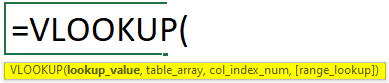
Arguments
- lookup_value – the value used as a reference while looking up
- table_array – is the table/range of the data within which we want to check specific values based on the lookup value.
- col_index_num – is the column number in the range of data from which we will get the values after lookup.
- Range_lookup – is an optional argument that specifies whether we need an exact matching value (FALSE) or approximate matching values (TRUE).
We will see some examples to specify how to compare two columns in Excel using the VLOOKUP function.
Examples of Compare Two Columns in Excel using VLOOKUP
we will discuss Examples of Compare Two Columns in Excel.
Example #1
Consider mixed data in columns A and B of the Excel sheet.
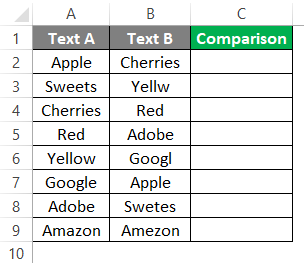
In column C, we need to check whether the values in column “Text B” match with those in “Text A”. Follow the steps below to get the comparison within these two columns using the VLOOKUP function.
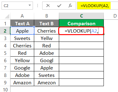
Step 1: Initiate the VLOOKUP function in cell C2 by typing “=VLOOKUP(“.
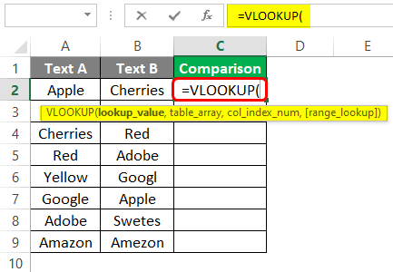
Step 2: The first argument we must specify is the lookup value. Since we are trying to determine whether the values from column Text A are present in a column named Text B, we need to specify the lookup value from column A. Since we are working with cell C2, using A2 as the lookup value is better. Separate it with a comma (“,”) to specify the next argument.
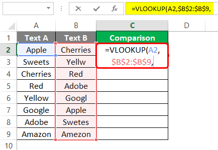
Step 3: The second argument for the VLOOKUP function is table_array. Which will be the range of data within which we wanted to check the values based on lookup_value. In our case, it is a column named Text B. Thus, select range from B2:B9 as a table_array and fix it using dollar signs so that the range will be the same for the formula when we copy it and paste it across different cells. You can use the keyboard shortcut F4 to fix the table range.
Step 4: Third and most important argument is to specify the column index from the table_array, which can be used to look up the values. Since only one column is selected as table_array, we can use the col_index_num value as 1.
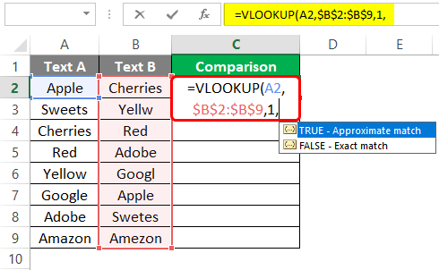
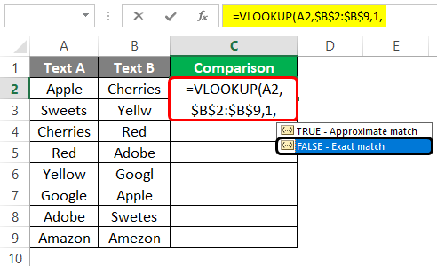
Step 5: The last argument is optional, which is range_lookup. Since it specifies whether we want an exact or approximate match, we can use TRUE (approximate match) or FALSE (exact match). We will be interested in exact matches; thus, we will use FALSE as the range_lookup argument.
We can also use the Boolean values for TRUE and FALSE as 1 and 0 under the VLOOKUP function, respectively.
Step 6: Use closing parentheses to complete the formula and press Enter to get the output. Note that if the function finds an exact match for the text in column A under column B, it will reflect the text; otherwise, it will reflect the #N/A error. Also, drag the formula across rows to get the formula applied for all cells.
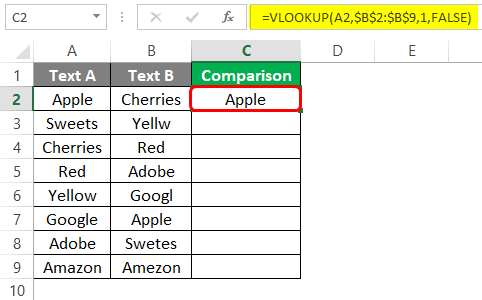
This is how we can compare two columns in Excel using the VLOOKUP function. However, the # N/A’s look not great in the data. It may look weird to someone who knows nothing about the formula/function. Let’s see another example where we try to get a more concrete solution for this issue.
Example #2
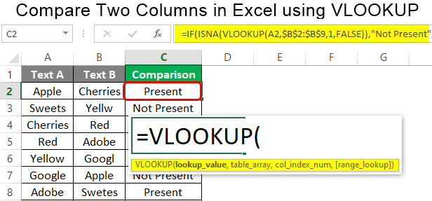
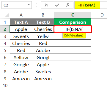
In this example, we will use conditional IF and ISNA with VLOOKUP to see whether the values from column A are present in column B.
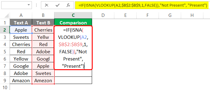
Step 1: Start the formula with “=IF(“and within it, use ISNA as a nested function as shown below:
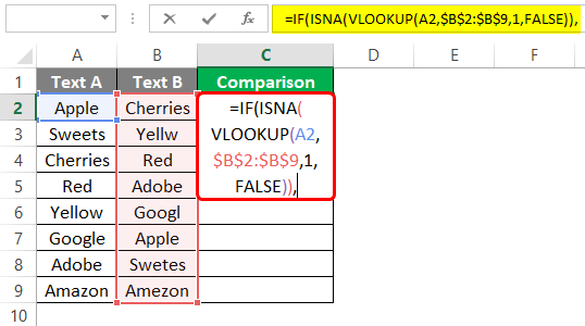
Step 2: Use the VLOOKUP function to check whether the values from column A are present in column B. same as we used in the first example. Close the parentheses for both VLOOKUP and ISNA functions. See the screenshot below for a better understanding.
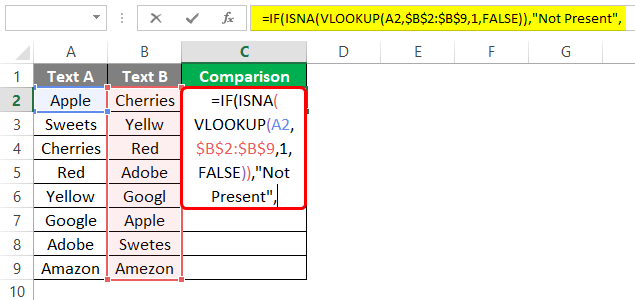
Step 3: We need to specify the values for the value_if_true argument for conditional IF. Specify it as “Not Present”. Don’t forget to use double quotes.
Step 4: For value_if_false, we need to specify the value. Use “Present” as a value for the argument. See the screenshot as shown below:
Step 5: Close the parentheses to complete the formula and press Enter button to get the output in cell C2. Also, drag the formula across the rows to get the desired output in terms of “Present” or “Not Present”. See the screenshot below for your reference.
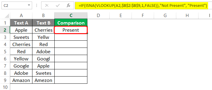
How does this work? Well, it is simple. Since ISNA checks whether the VLOOKUP returns #N/A or not, if there are any #N/A, the function returns TRUE, and thus IF function has “Not Present” as an argument for this output. Similarly, if ISNA doesn’t find #N/A, then the value it returns is FALSE, and we have “Present” as an argument under the conditional IF statement.
Thus, wherever we are getting Not Present, those values from column A don’t have to match in column B.
We will wrap this article to end it here. However, we have some points to remember for you all.
Things to Remember
- When comparing values within two columns, VLOOKUP does not require the values to be ordered.
- If VLOOKUP doesn’t get the match for lookup_value under table_array, it returns by default as a #N/A error.
- We can combine VLOOKUP with IF and ISNA to generate a more versatile result where no #N/A gets reflected within the data for those values which doesn’t match.
Recommended Articles
This has been a guide to Compare Two Columns in Excel using VLOOKUP. Here we discuss How to Compare Two Columns in Excel using VLOOKUP and practical examples. You can also go through our other suggested articles –
