Updated June 9, 2023
RATE Formula in Excel
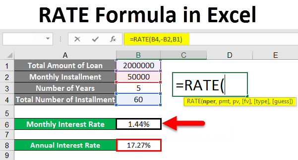
This Rate Formula in Excel provides the interest rate of a period per annuity. The RATE function repeatedly calculates to find the rate for that period. The RATE function can be used to find a period’s interest rate and then multiplied to find the annual interest rate. So this formula can be used to derive the interest rate. The formula of this function is as follows.
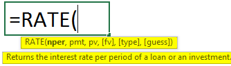
=RATE(nper, pmt, pv, [fv], [type], [guess])
Below is the explanation of the given arguments:
- nper – No. Of Payment periods for an annuity. (Required)
- pmt – Payment to be made for each period; this will be fixed. (Required)
- pv – Present Value, Total Amount that a series of future Payments worth now. (Required)
- fv – Future Value, Goal amount to have after the subsequent Instalment; if we exclude fv, we can take 0 instead. (Optional)
- type –
- This examines how the function will consider the payment due date, so we have to put this in binary 0 or 1; 0 means payment is due at the end period. (Optional)
- guess – This argument is used for our guess of the interest rate. It will provide the rate function with a start before reaching 20 iterations. There were two possibilities for this argument when it assumes our guess as 10%; otherwise, it will attempt other values for input(Optional).
How to Use RATE Formula in Excel?
We will now learn how to write the RATE formula to get the lookup value. Let’s understand this formula with some examples.
Example #1
- For this example, suppose you want to buy a car, and the price of that car is INR 3,00,000.00. And you
went to a banker and asked for a car loan; you were told that you have to pay INR 10,000.00 per
month for 3 years (36 Months)
- Here is the situation where we can use our RATE function to find the Interest rate for the given
condition.
- Now, as per the below image, you can see that we have mentioned the details we have, Now initially
we will find the interest rate per month and then for a year by multiplying it by 12.
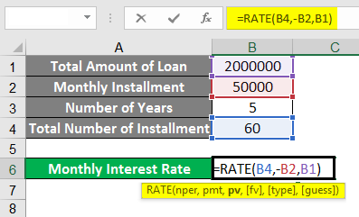
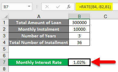
Now you can see from the below image you can see that we have applied the formula for RATE is as
follows:
=RATE(B5, -B3, B2)
Here are the arguments :
nper = B5 (Total no. Of Instalments)
pmt= -B3 (Payment for each Instalment)
pv= B2 (Loan Amount)
- Here you can notice that the pmt (B3) is taken negatively because the calculation is from the borrower’s
perspective, so this is the monthly installment amount which is the cash outflow for the individual
(Borrower) must pay every month. So the borrower is losing this amount every month; that’s the
cause why it’s negative.
- Now here, if we calculate this loan from the bank’s perspective, as the bank is giving this loan on a monthly basis to the borrower, the (B2) loan amount will be negative because on every Instalment the bank has to pay that less to the borrower monthly, so as per the perspective we have to change the negative sign in the formula.
- Now you can see that by using this function, we have found the monthly interest rate (In our case, it’s 1.02%).
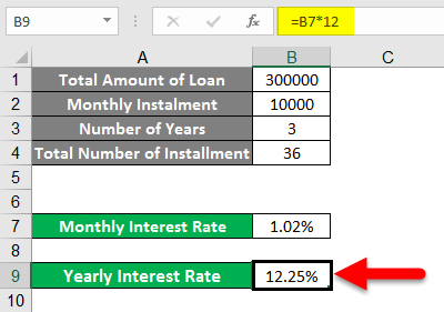
- And by multiplying it by 12, we can have the rate of interest annually (In our case, it’s 12.25%).
Example #2
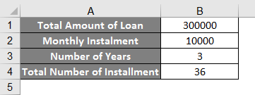
- Similar to the above example for the practice, we will see another example where we have to find the interest rate. As per the below image, we have the data to find the interest rate.
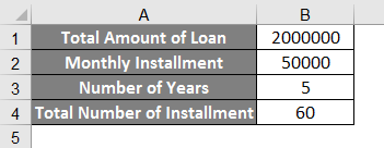
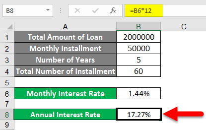
- Here we have 20 Lacs to pay with 50 thousand per month for 5 years (60 Instalments).
- So the arguments are as follows:
nper = 20 Lacs
pmt = 50,000
pv = 60 Instalments (5 years)
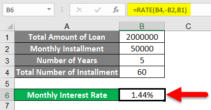
- As per the above image, we can see that the RATE function has been applied and found the monthly rate of interest is 1.44%
- By multiplying it by 12, we will get the annual interest rate of 27% for the given example.
Example #3
- For this example, suppose we know the interest rate and not the installment, but we want to find out the monthly installment amount.
- Here for this example, we have taken the following data as per the below image:
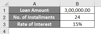
- We have taken a loan of 3 Lacs at a 15% of interest rate (Annually); here, we know the interest rate, but we need to find the pmt: Amount Payable for each Instalment.
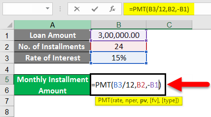
- Here as we can see from the image below, the formula for pmt is as follows :
=pmt(B4/12, B3, -B2)
- We can notice that we have taken the B4/12 because the rate of interest provided to us is per annum (annually), so by dividing it by 12, we are making it monthly.
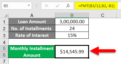
- So as we can see in the below image, the monthly installment amount will be $14,545.99, to be exact.
- As per the above example, we have found one of our arguments for the RATE function.
Things to Remember about RATE Formula
#NUM! Error:
This error can occur when the rate result does not converge within 0.0000001 for 20 iterations. It can happen when we don’t mention cash flow convection by assigning the negative sign to the appropriate argument in the formula; as per the above example, we have seen that when we calculate the rate for the borrower side, the monthly installment amount getting negative sign because of monthly cash outflow for the borrower. So if we didn’t apply that negative sign to the monthly cash outflow, we would encounter this error.
- So here, we can put the guess argument to work because it will allow us to start as it converges within 20 iterations and provide us with the closing or even the correct answer.
- All arguments should be numeric; otherwise, they will encounter the #value error.
- With the RATE function, when calculating the interest rate for the given data, we will find the interest rates per month. So to convert it to annual interest, we must multiply it by 12.
Recommended Articles
This has been a guide to the RATE Formula in Excel. We discussed using the RATE Formula in Excel, practical examples, and a downloadable Excel template here. You can also go through our other suggested articles –
