Updated June 6, 2023
What is 3D Cell Reference in Excel?
3D Reference in Excel allows users to choose the same cell from different and multiple worksheets. To use reference in Excel, we can choose the same cell or range of cells from different sheets by selecting the worksheet’s name. For example, we have 3 worksheets with different number values, and the name of the worksheets are First Second, and Third. Now, if we want to sum the values of this worksheet without selecting the cell from there, we can use their names like FIRST: THIRD with the cell with want to add. If we want to sum the value of cell location A1, we must use the range in the SUM function as FIRST: THIRD!A1.
How to Use 3D Cell Reference in Excel?
The best way to learn a concept is through examples. Let us take a look at a few examples to get a better understanding.
Example #1
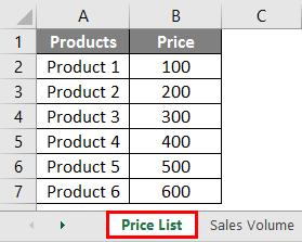
- Let us assume we have a list of prices for a group of products in Sheet 1, which has been renamed “Price List”, as shown below.
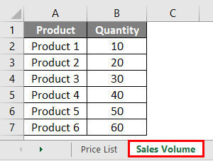
- Now, we also have the number of products sold or the Sales Volume defined in another tab – Sheet 2, which has been renamed to Sales Volume.
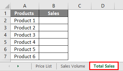
- Now we wish to calculate the total sales for each product in Sheet 3, renamed Total Sales.
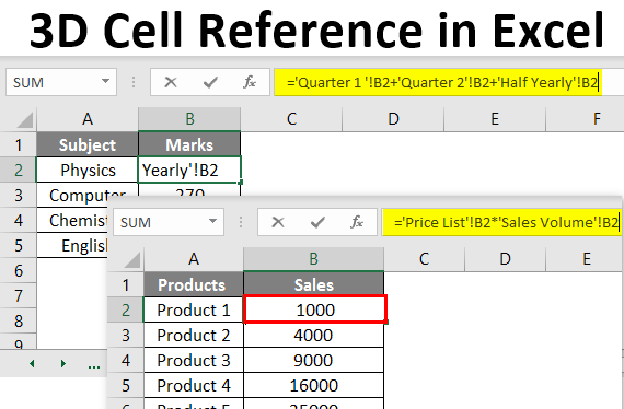
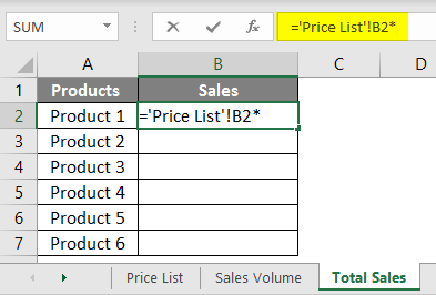
- The next step is to go to Cell B2 and type the formula = after this, we need to change the reference to sheet 1, where the price list is defined. Once the cell reference has been set, we will need to select the price for the first product; in this case, it is Product 1.
![]()
- As we can see, in the function bar, we have the cell reference pointing to the Price List sheet, which is the first sheet. On closer examination, it refers to the Price List sheet and cell B2, the Sales of Product 1.
- Now we need to put an asterisk (*) in the formula. Asterisk is the symbol for multiplication. We need to multiply Sales by the number of products sold to calculate the total sales for a product.
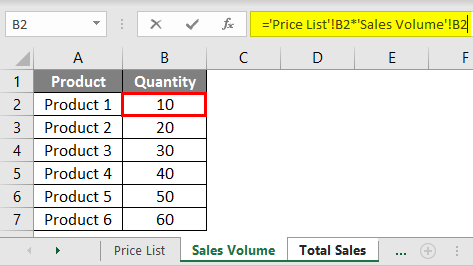
- We need to change the cell reference to the second sheet – Sales Volume. Once we have changed the cell reference, we must select Quantity for Product 1.
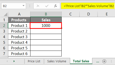
- Now we need to drag the formula to the rest of the rows in the table, and we will get the results for all the other products.
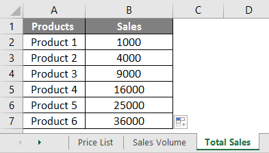
- So basically, in the above example, we successfully gave references from two different sheets (Price List and Sales Volume) and pulled the data to calculate the total sales in a third sheet (Total Sales). This concept is called 3D Cell Reference.
Example #2
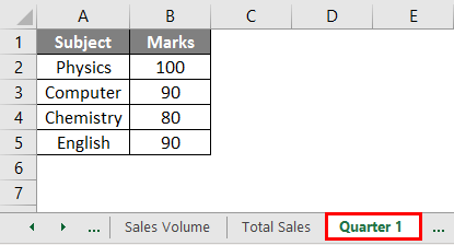
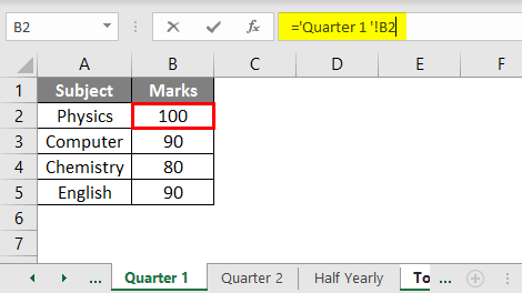
- Now suppose we have a student’s data. We have his half-yearly and quarterly test scores for five subjects. Our objective is to calculate the total marks in a third sheet. So, we have the quarterly test scores for a student in five subjects, as shown below.
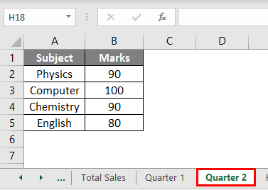
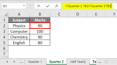
- We also have the Quarter 2 test scores, as shown below.
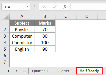
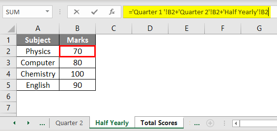
- We also have the Half Yearly test scores, as shown below.
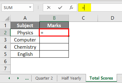
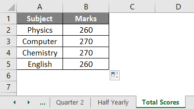
- Now we wish to calculate the total test scores in another worksheet using 3D Referencing in Excel. To do that, we will apply the formula as follows:
- First, we shall write “=” for Marks in the Total Scores tab for the first subject, i.e., Physics.
- Next, we shall change the cell reference to Quarter 1 and then select the marks for Physics from that tab.
- Next, we shall add a “+” sign in the formula to add the next item to the Quarter 1 score. To do this, we shall change the cell reference using the 3D reference to the Quarter 2 tab and select the Quarter 2 marks for physics.
- Next, we shall again add the “+” sign to the formula to add the next item, i.e., the Half Yearly score. To do that, we shall again change the cell reference by using the 3D reference to the Half Yearly tab and select the half-yearly score for Physics.
- Now that we have the summation of all the scores for this student in Physics, we shall press enter key to get the total score.
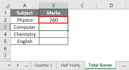
- Now, we shall drag this formula to the rest of the rows in the table to replicate the summation across all the subjects.
Example #3
- So far, we have seen a 3D reference for performing calculations. But we aren’t limited to just that. We can use the 3D reference to make charts and tables as well. In this example, we shall demonstrate how to create a simple chart using this concept.
Suppose we have the sales data for a company.
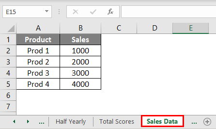
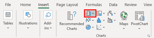
- We shall use this data to create a simple chart in another worksheet. So, we shall create a new tab, rename it to “Chart”, and go to the Insert tab in the ribbon on the top. Here, we shall select the Insert Column or Bar chart.
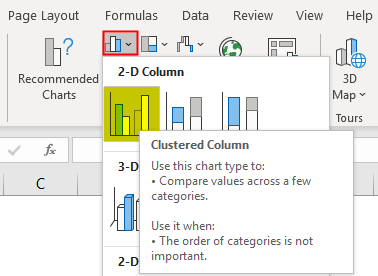
- Next, we shall select a simple 2-D Clustered Column chart.
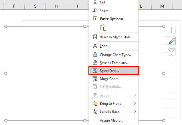
- Now, right-click on the chart area and select “Select Data….”
- We shall get a dialog box to select the chart data source.
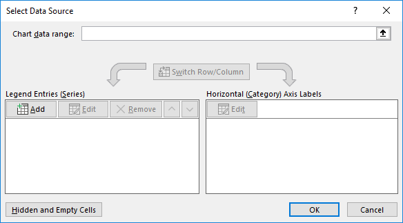
- Here we shall select the source data from the Sales Data tab. We shall select the range of cells where we have defined the Sales for each product.
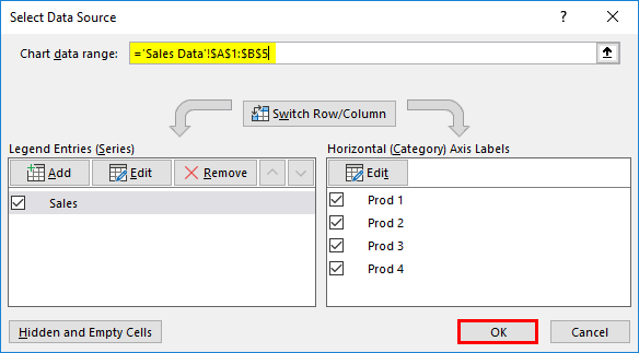
- We notice here that all our listed products are mentioned on the right pane of the dialogue box. This shows the source data selection. We can edit the source data as required by clicking the “Edit” button above this pane.
- After this, we shall click OK, and our chart will be created in the “Chart” tab.
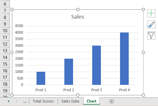
Thus, we have successfully created the chart by using the 3D reference.
Things to Remember
- The data must be in the same format or pattern in all the tabs.
- Even if the referenced worksheet or the cells in the referenced cell range are altered, moved, or deleted, Excel will continue to refer to the same reference. In case of alterations, moving, or deletion, it will result in the cell reference evaluating to NULL if appropriate values are not found.
- Even if we add one or more tabs between the referenced and final worksheets, it will change the result as Excel will continue to refer to the original reference provided.
Recommended Articles
This is a guide on 3D Cell Reference in Excel. Here we discuss How to Use 3D Cell Reference in Excel with different examples and the downloadable Excel template. You may also look at the following articles to learn more –
