Updated August 10, 2023
Mixed Reference in Excel (Table of Contents)
Introduction to Mixed Reference in Excel
Mixed References in Excel is used to fix either column or row simultaneously. It refers to the only Column or Rows of the referred cell. By this, any of the references can be fixed.
For example, if we want to apply mixed reference in a cell, say A1, then we can fix the column of cell A1 by putting dollar(“$”) before the column name $A1 or to fix the row of cell A1 then we can put dollar before the cell number A$1. In short, when we put $ before anything, it locks it.
Examples of Mixed Reference in Excel
Here are the examples of Relative and Absolute Reference work with Mixed Reference in Excel below.
Example #1 – Relative Reference
By default, the reference in Excel will consider a Relative reference. Reference is nothing if we input “=A1” in cell B1, then we are referring to A1 in B1. Let’s see an example to understand the relative reference.
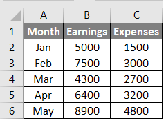
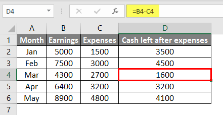
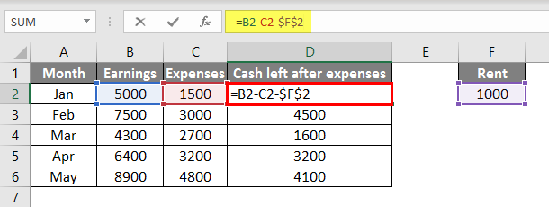
Consider the below screenshot of earnings and expenses from Jan to May.
Now we want to calculate the cash left after the expenses paid from the earnings. We can get that with the simple formula of subtraction of expenses from the earnings. Just input the formula next to expenses to find the remaining monthly cash.
Observe the below screenshot I have input the formula next to expenses which you can find from the formula bar.
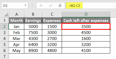
If we observe that the formula in D2 is B2-C2, D2 refers to the combination of B2 and C2. When we drag the formula to the bottom lines, it will take a similar to D2, which means D2 takes reference from B2 and C2, similarly for D3, it will take reference from B3 and C3, For D4 take reference from B4 and C4, and so on.
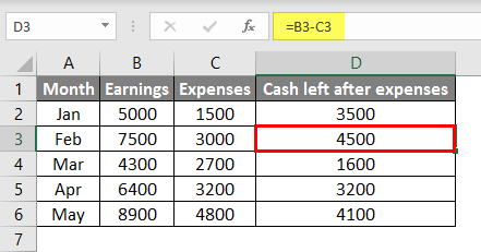
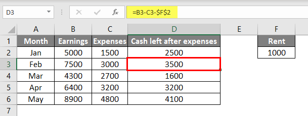
We can observe the related screenshots for other months. The below screenshot is D3 related, which refers to B3 and C3.
D4-related screenshot, which refers to B4 and C4.
That means the formula will always consider the same reference as the first formula related to that. I hope you got an idea of what is a relative reference where we can use it.
Example #2 – Absolute Reference
Consider the same example to understand Absolute reference also. Let us consider from the above screenshot we have earnings and expenses; let’s assume we have fixed rent expenses and the expenses available in the table.
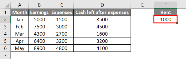
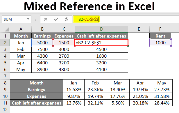
In the above Excel, we mentioned rent in only one cell, F2. Now we need to amend the formula in column D to subtract rent from the “cash left after expenses”.
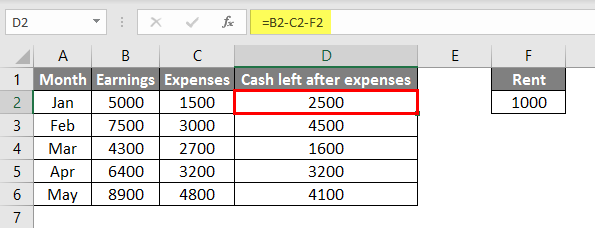
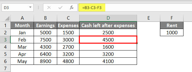
Observing the screenshot, we subtracted F2 from the result of B2-C2. Let’s drag the formula to the other cells, also.
I dragged the formula, but the results did not change because, in cell D2, we subtracted F2 as explained earlier; by default, Excel will take relative reference, so it took F3 for the formula in D3, similarly F4 in D4. But we do not have any values in the cells F3, F4, F5, and F6; that is why it considers those cells zero and did not affect the results.
We can solve this without dragging rent to F3, F4, F5, and F6. Here Absolute reference helps to achieve the correct results without dragging the rent.
It is very simple to create the absolute reference; we need to click on the formula, select the cell F2, and click D2. Then the absolute reference will create.
If $ is applied for column index F and row index 2, then the absolute reference is at the cell level. Now drag the formula in D3, D4, D5, and D6 and see how the results change.
Observe the formula in cell D3; it is $F$2 only even after we dragged the formula. As it is locked at the cell level, it will take reference from F2 only. This is the use of absolute reference. This will take the reference from the locked index.
Example #3 – Mixed Reference
As mentioned earlier, we will use both relative and absolute reference in mixed reference. Let’s see how we can use both using the same example.
Consider the data in the below format, as shown in the screenshot.
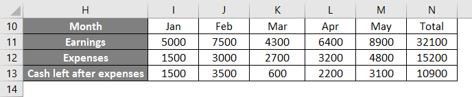
From the above table, we need to find the percentage of each month’s earnings against the “Total” of 5 months’ earnings, similarly, percentages for expenses and cash left after expenses.
If still unclear, we need to find 5000 percent out of the total 5 months’ earnings of 32100.
Now in the below empty table, we need to find the percentage for each cell.
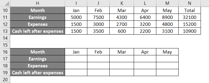
The formula for finding the percentage is divided by Jan’s earnings with a total of 32100.
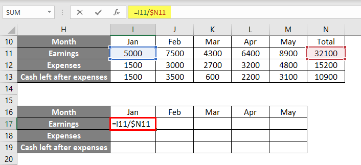
If you observe, I have used the absolute reference because all month’s earnings should divide by the total only. Now we can drag the formula until May.
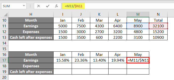
Now drag the formulas to the bottom also.
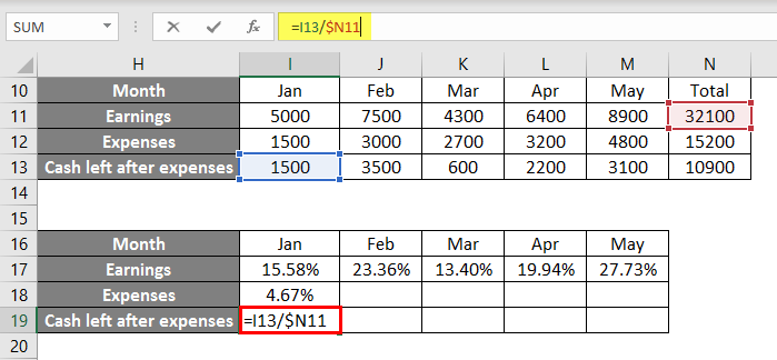
If we observe still, the formula for expenses is taking a total of Earnings only, but actually, it should take expenses total of 15200. For that, we need to create a reference at the column level alone, not required at the row level.
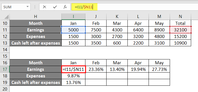
Observe that the formula $ symbol is available at N, not row index 11. Make the changes always to the first formula, then drag to the other cells.
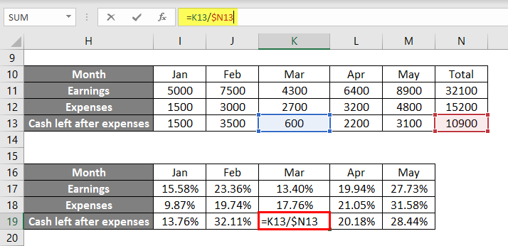
Everywhere the formula is picking correctly. If we observe, we performed the absolute reference in row operations and relative reference in column operations. I hope now it is clear how to perform mixed reference and in which areas it will be useful.
Things to Remember
- A mixed reference is a combination of relative reference and absolute reference.
- Relative reference is a default reference in Excel while referring to any cells in Excel operations. This other cell will take a similar reference as the first formula.
- An absolute reference is another type that will take the reference as fixed where ever you paste the formula.
- To create an absolute reference, select the cell reference and click on F4; then, the $ symbol will add to the row and column indexes.
- Mixed reference combines both; hence, we may apply an absolute reference to the column or row indexes alone.
- $A1 – Means reference created for column index.
- A$1 – Means reference created for row index.
- $A$1 – Means reference created for both row and column indexes.
Recommended Articles
This is a guide to Mixed Reference in Excel. Here we discuss How Relative and Absolute References work with Mixed References in Excel, examples, and a downloadable Excel template. You may also look at the following articles to learn more –
