Updated June 13, 2023

Introduction to Survival Analysis in R
Survival Analysis in R estimates the lifespan of a particular population under study. It is also called ‘Time to Event Analysis’ as the goal is to predict the time when a specific event will occur. It is also known as the time-to-death analysis or failure time analysis. As an example, we can consider predicting the time of death of a person or predicting the lifetime of a machine. From any company perspective, we can view the birth event as when an employee or customer joins the company and the respective death event as when an employee or customer leaves that company or organization.
Data: Survival datasets are time-to-event data that consists of distinct start and end time. In real-time datasets, all the samples do not start at time zero. A sample can enter at any point in time for study. So subjects are brought to the common starting point at time t equals zero (t=0). When the data for survival analysis is too large, we need to divide the data into groups for easy analysis.
Survival analysis is of significant interest for clinical data. With the help of this, we can identify the time to events like death or recurrence of some diseases. It is helpful for the comparison of two patients or groups of patients. The data can be censored. The term “censoring” means incomplete data. Sometimes a subject withdraws from the study, and the event of interest has not been experienced during the whole duration of the study. In this situation, when the event is not experienced until the last study point, that is censored.
Necessary Packages
The necessary R survival analysis packages are “survival” and “survminer.” For these packages, the version of R must be greater than or at least 3.4.
- Survival: For computing survival analysis
- Survminer: For summarizing and visualizing the results of survival analysis.
The package name “survival” contains the function Surv(). This function creates a survival object. We use the survfit() function to create a plot for analysis.
The basic syntax in R for creating survival analysis is as below:
Surv(time,event)

survfit(formula)
Where,
Time is the follow-up time until the event occurs. The event indicates the status of the occurrence of the expected event. The formula is the relationship between the predictor variables.
Types of Survival Analysis in R
There are two methods mainly for survival analysis:
- Kaplan-Meier Method and Log Rank Test: You can implement this method using the survfit() function and use plot() to graph the survival object. You can also use the function ggsurvplot() to plot the survfit object.
- Cox Proportional Hazards Models coxph(): We use this function to obtain the survival object and employ ggforest() to plot the graph of the survival object. This is a forest plot.
Implementation of Survival Analysis in R
First, we need to install these packages.
install.packages(“survival”)

install.packages(“survminer”)
To fetch the packages, we import them using the library() function.
library(“survival”)

library(“survminer”)
Let’s load the dataset and examine its structure. For survival analysis, we will use the ovarian dataset. We use the data() function in R to load the dataset.
data(“ovarian”)
The ovarian dataset comprises ovarian cancer patients and respective clinical information. The tracking period also encompasses the time until patients either died or became lost to follow-up. It indicates whether we censored patients or not, their age, assigned treatment group, presence of residual disease, and performance status.
To inspect the dataset, let’s perform head(ovarian), which returns the initial six rows of the dataset.
head(ovarian)
Output:
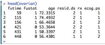
Here, the columns are- futime – survival times fustat – whether survival time is censored or not age - age of patient rx – one of two therapy regimes resid.ds – regression of tumors ecog.ps – performance of patients according to standard ECOG criteria. Here as we can see, age is a continuous variable. So this should be converted to a binary variable. What should be the threshold for this? Let’s compute its mean so that we can choose the cutoff.
mean(ovarian$age)
Its value is equal to 56. We are here taking 50 as a threshold. We will consider age>50 as “old” and otherwise as “young.”
ovarian <- ovarian %>% mutate(ageGroup = ifelse(age >=50, "old","young"))

ovarian$ageGroup <- factor(ovarian$ageGroup)
Now we will use Surv() function and create survival objects with the help of survival time and censored data inputs.
survObj <- Surv(time = ovarian$futime, event = ovarian$fustat)

survObj
Output:
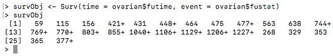
Here the “+” sign appended to some data indicates censored data.
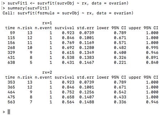
Now to fit Kaplan-Meier curves to this survival object, we use the function survfit(). We can stratify the curve based on the treatment regimen ‘rx’ assigned to patients. The summary() function of the survfit object displays the patients’ survival time and proportion.
survFit1 <- survfit(survObj ~ rx, data = ovarian)

summary(survFit1)
Output:
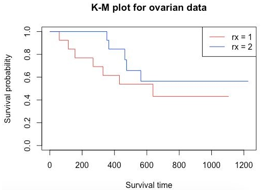
To view the survival curve, you can use the plot() function and pass the survFit1 object. To add a legend to the plot, simply use the legend() function.
plot(survFit1, main = "K-M plot for ovarian data", xlab="Survival time", ylab="Survival probability", col=c("red", "blue"))

legend('topright', legend=c("rx = 1","rx = 2"), col=c("red","blue"), lwd=1)
Output:
Now let’s take another example from the same data to examine the predictive value of residual disease status.
survFit2 <- survfit(survObj ~ resid.ds, data = ovarian)

plot(survFit2, main = "K-M plot for ovarian data", xlab="Survival time", ylab="Survival probability", col=c("red", "blue"))

legend('topright', legend=c("resid.ds = 1","resid.ds = 2"), col=c("red", "blue"), lwd=1)
Output:
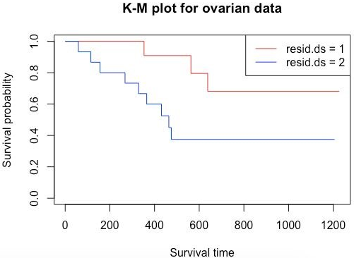
Here as we can see, the curves diverge quite early. Here considering resid.ds=1 as less or no residual disease and one with resid.ds=2 as yes or higher disease, we can say that patients with the less residual disease have a higher probability of survival. Now let’s do a survival analysis using the Cox Proportional Hazards method. Using coxph() gives a hazard ratio (HR). If HR>1, then there is a high probability of death; if it is less than 1, then there is a low probability of death.
survCox <- coxph(survObj ~ rx + resid.ds + age_group + ecog.ps, data = ovarian)

ggforest(survCox, data = ovarian)
First, we need to change the labels of columns rx, resid.ds, and ecog.ps to consider them for hazard analysis.
ovarian$rx <- factor(ovarian$rx, levels = c("1", "2"), labels = c("A", "B"))

ovarian$resid.ds <- factor(ovarian$resid.ds, levels = c("1", "2"),

labels = c("no", "yes"))

ovarian$ecog.ps <- factor(ovarian$ecog.ps, levels = c("1", "2"), labels = c("good", "bad"))
Output:
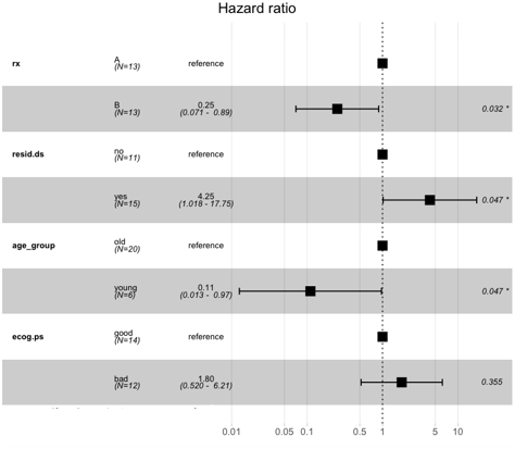
Here we can see that the patients with regime 1 or “A” have a higher risk than those with regime “B.” Similarly, the one with younger age has a low probability of death, and the one with higher age has a higher death probability.
Recommended Articles
This is a guide to Survival Analysis in R. Here; we discuss the basic concept with necessary packages and types of survival analysis in R and its implementation. You may also look at the following articles to learn more –
