Updated August 19, 2023
Introduction to Superscript in Excel
Superscript in Excel is used to put the number or text in small fonts above the base numbers and text. It is like giving power raised to any base number as we do in mathematics. It is like using superscript to write the text in the square of base units or text such as Feet2, Meter2, etc. Likewise, we can use superscript numbers, such as 102 or 25. Superscript is not a function in Excel. It is mainly made for MS Work which deals with text. To activate this, go to the edit mode of any cell and select Format Cells from the right-click menu. And from there, we can tick Superscript from the Fonts tab.
Examples of Superscripts
X2, ab,2nd, sin2(30)
- X2 – Here, the superscript is ‘2’, a number for its previous character X.
- Here, the superscript is ‘b’, a character for its previous character.
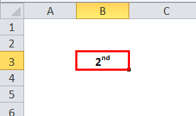
- 2nd – Here, the superscript is ‘nd’, a string for its previous number 2.
- Sin2(30) – The superscript is ‘2’, a number for its previous string ‘sin’.
I hope you all understand what superscript is. Let’s begin with how to do it in Excel.
Steps to get a Superscript Text in Excel
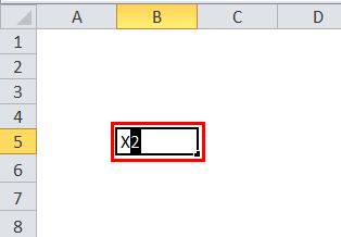
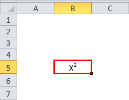
It is easy to input superscript text in Excel; follow these simple steps. Let’s try to input X2.
Input X2 in any of the cells where you require the superscript. Now select number 2 alone by clicking F2 and select 2 or double-click on the cell and select 2 alone.
I am giving the screenshot for a better understanding.
Method #1
Once you select the number 2 and right-click the mouse, a pop-up will appear, as shown in the picture below.
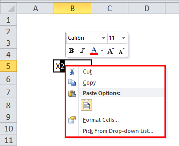
From the popup menu, select Format cells.
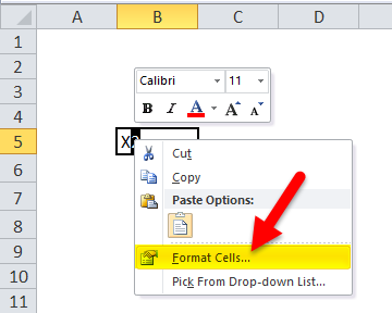
Then the “format cells” menu will appear.
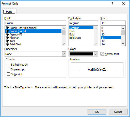
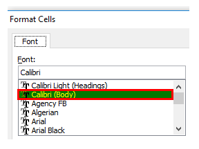
From the menu “Font”, we can select the required font for the superscript.
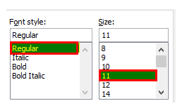
From the menu “Font style” and menu “Size”, we can select the required font style for the superscript like Italic, bold, and required Size, etc.
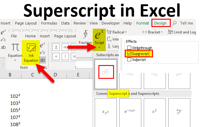
From the menu “Effects”, we can select the option superscript.

After selecting the superscript, select “ok”, then you can find the number 2 will be on the top of X as a superscript of X.
Similarly, you can perform superscript text for other examples.
For your better understanding, find the below screenshots for one more example.
Method #2
First, give the “2nd” in an Excel cell.

Select “nd” alone and do right-click. Then select “format cell” and “superscript” as marked.

The result is:
How to Use Superscript in Excel?
This superscript and subscript feature is helpful while working with Mathematical or scientifically related data.
We have a few more ways to input superscript text in Excel.
Superscript in Excel Example #1 -Through Quick access toolbar(QCT)
We can input superscripts through QCT, also. Here are the steps on how to do that.
For people who are not aware quick access toolbar, below is the screenshot.
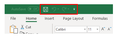
Currently, we have “Save”, “Undo”, and “Redo”; hence we need to add the “Superscript” option to QCT.
Click on the “File” menu the following dropdown menu will appear. From that drop-down menu, select “Options”.

When you click “Options”, another screen will appear, as shown below.
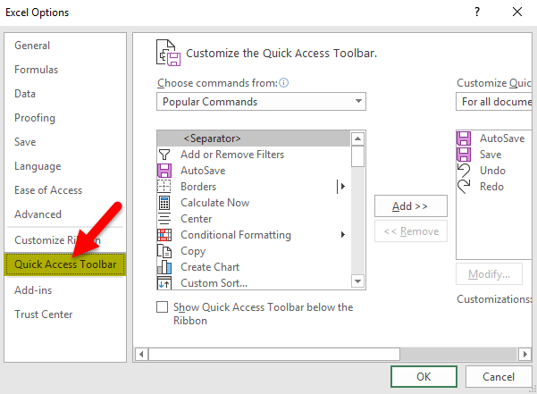
Select “Quick Access Toolbar” from the above screen, highlighted left-hand. We can observe there are multiple numbers of commands available in the rectangle screen. One can scroll, select the required commands and click on “Add” to add to the QCT as we required the Superscript command, search for that, select superscript, and click on Add.
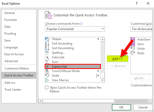
Once you click “add”, the superscript will move from the left to right side QCT rectangular box.
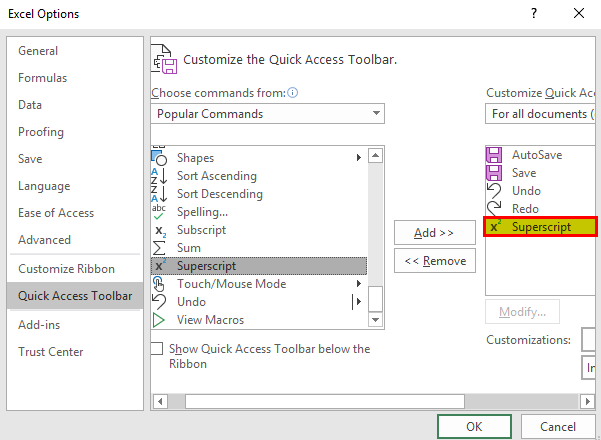
And then click on the “Ok” button at the bottom; the menu will close and return to Excel.
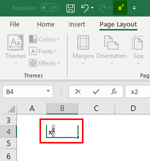
Now we can observe the QCT; an additional option is visible that is x2 marked in the picture.
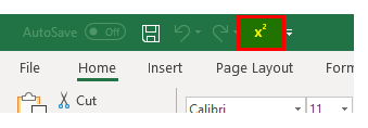
It is easy to input superscript; select the letter or text you want to convert as superscript and click on the X2 option in the Quick Access toolbar.
If you want to remove the superscript, reselect the X2 command, then it will be converted to the normal text again.
Superscript in Excel Example #2 – Applying Superscript for Number
Whatever process we discussed will not work for numbers, i.e., 25. you can try both ways, whether from QAT or from right-click. The movement you move from the cell will convert to normal numbers.
To apply superscript for numbers, follow the below steps.
Click on the “Insert” at the top. If we observe the righthand side, we can observe the option” Equation”, which is marked.
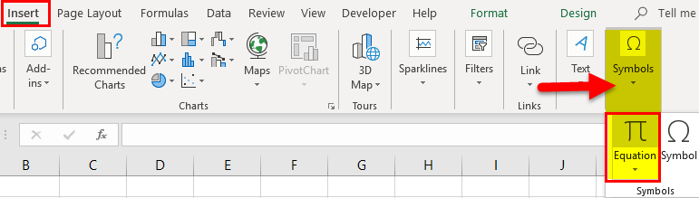
Click on the option “Equation”, and then the menu changes to the design.

Click on the “ex” option, which is marked then the dropdown will come from that drop-down select the format for superscript, which I marked in the below picture.
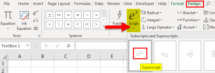
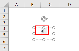
We can observe a pattern in the cell, as shown in the below picture.

Select the first cell and give the Base number and then select the small box at the top to give the power.
Superscript in Excel Example #3
Another way is when you click on the “Equation”, it will take you to the “design” menu. We can observe the “Ink Equation” option on the left-hand side.
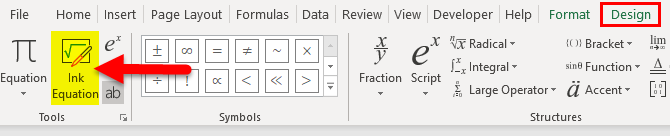
Once you click “Ink Equation”, another screen will pop up there; you can manually write the required text using your mouse. Once your text is over, click on “Insert” at the bottom of the box.
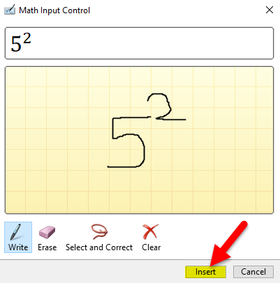
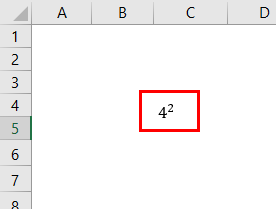
The Output is:
Superscript in Excel Example #4 – Superscript for multiple numbers at a time
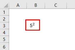
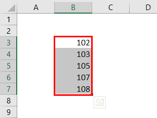
Select the range of numbers you want to give a similar superscript number. Let’s take the example of 5 numbers to which we want to apply superscript 2.
Select all 5 numbers.
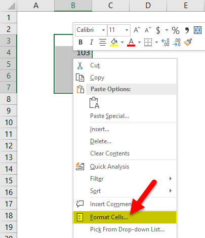
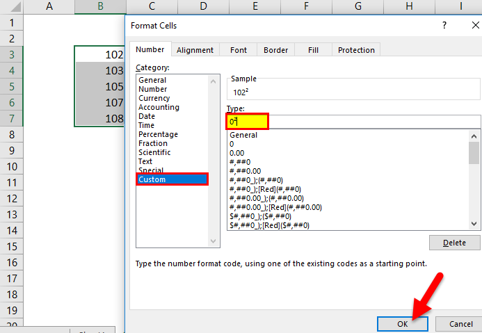
Now right-click, and a popup will come up. From that popup, choose format cells.
After that, select “custom” at the bottom and select “zero,” as marked in the picture.
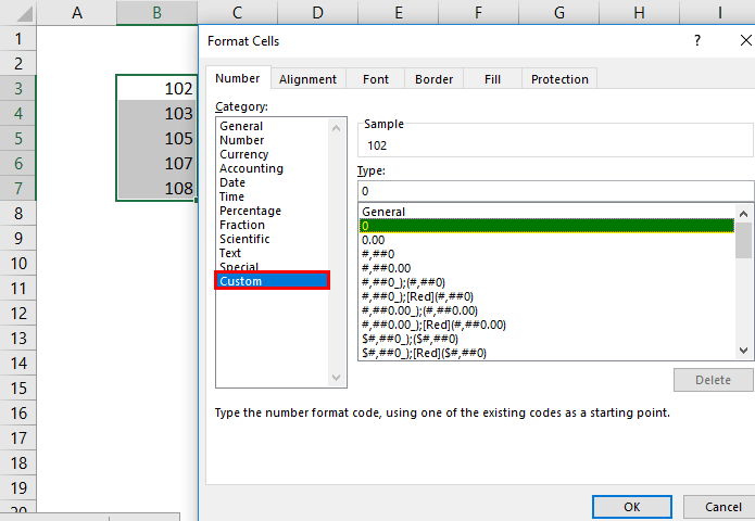
Keep the cursor at zero.
Hold the ALT key and give 0178; then zero becomes zero square. Then click on “Ok”.
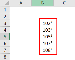
Now we can check the Excel sheet; all the selected numbers have Power 2.
Similarly, we can input superscripts 1 and 3 also.
Shortcut for 1 is held ALT + 0185
Shortcut for 3 is held ALT+ 0179.
Shortcut for Superscript
If we want to input superscript text with a keyboard shortcut, then it is very easy. Input the required text in the Excel cell, select which you want to convert as superscript, and then press the ALT button from the keyboard.
The superscript option on the Quick Access toolbar will highlight a number as shown below:

Observe that number and click that number on the keyboard. Here it is 5 marked in the above picture for reference.
Things to Remember About the Superscript in Excel
In Excel, users utilize superscripts to input mathematical and scientific data. a. Superscripts can be input in multiple ways, but those ways are unsuitable for a number format. Use the special process for numbers alone, as discussed above. When an input for the number, it will not give any results; it is just for representation purposes. Subscript is also quite similar to superscript. One can also try subscript with the help of the above methods.
Recommended Articles
This has been a guide to a Superscript in Excel. Here we discuss its uses and how to use Superscript in Excel with Excel examples and downloadable templates. You may also look at these useful functions in Excel –