Updated March 21, 2023
Introduction to Simple Linear Regression
The following article provides an outline for Simple Linear Regression.
From Dictionary: A return to a former or less developed state.
In Statistics: A measure of the relation between the mean value of one variable and corresponding values of the other variables.
The regression, in which the relationship between the input variable (independent variable) and target variable (dependent variable) is considered linear, is called Linear regression. Simple Linear Regression is a type of linear regression where we have only one independent variable to predict the dependent variable. Simple Linear Regression is one of the machine learning algorithms. Simple linear regression belongs to the family of Supervised Learning. Regression is used for predicting continuous values.
Model of Simple Linear Regression
Let’s make it simple. How it all started?
It all started in 1800 with Francis Galton. He studied the relationship in height between fathers and their sons. He observed a pattern: Either the son’s height would be as tall as his father’s height, or the son’s height would be closer to all people’s overall avg height. This phenomenon is nothing but regression.
Example:
Shaq O’Neal is a very famous NBA player and is 2.16 meters tall. His sons Shaqir and Shareef O’neal are 1.96 meters and 2.06 meters tall, respectively. The average population height is 1.76 meters. Son’s height regress (drift toward) the mean height.
How we do Regression?
Calculating a regression with only two data points:

We want to find the best regression to draw a line that is as close to every dot as possible. In the case of two data points, it’s easy to draw a line; just join them.
Now, if we have a number of data points now, how to draw a line that is as close as possible to each data point.
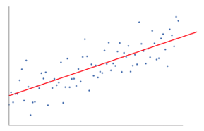
In this case, our goal is to minimize the vertical distance between the line and all the data points. In this way, we predict the best line for our Linear regression model.
What Simple Linear Regression does?
Below is a detailed explanation of Simple Linear Regression:
- It draws lots and lots of possible lines of lines and then does any of this analysis.
- Sum of squared errors.
- Sum of absolute errors.
- Least square method…etc.
- For our analysis, we will be using the least square method.
- We will make a difference of all points and calculate the sum of all the points. Whichever line gives the minimum sum will be our best line.
Example: By doing this, we could take multiple men and their son’s height and do things like telling a man how tall his son could be. Before he was even born.
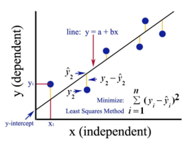
Google Image
The above figure shows a simple linear regression. The line represents the regression line. Given by: y = a + b * x.
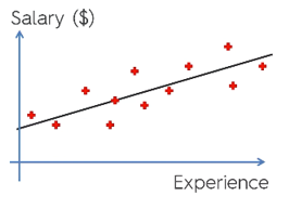
Where y is the dependent variable (DV): For e.g., how the salary of a person changes depending on the number of years of experience that the employee has. So here, the salary of an employee or person will be your dependent variable. The dependent variable is our target variable, the one we want to predict using linear regression.
x is our independent variable (IV): The dependent variable is the cause of the change independent variable. In the above example, the number of years of experience is our dependent variable because the number of years of experience is causing the change in the salary of the employee.
- b is the coefficient variable for our independent variable x. This coefficient plays a crucial role. It says how a unit change in x (IV) is going to affect y (DV). It is referred to as the coefficient of proportionate also. In terms of mathematics, it is up to you as the line’s slope, or you can say steep of the line.
- In our example, if slope (b) is less, which means the number of years will yield less increment in salary; on the other hand, if the slope (b) is more will yield a high increase in salary with an increase in the number of years of experience.
- a is a constant value. It is referred to as intercept also, which is where the line is intersecting the y-axis or DV axis. In another way, we can say when an employee has zero years of experience (x), then the salary (y) for that employee will be constant (a).
How does Least Square Work?
Below are the points for least square work:
- It draws an arbitrary line according to the data trends.
- It takes data points and draws vertical lines. It considers vertical distance as a parameter.
- These vertical lines will cut the regression line and gives the corresponding point for data points.
- It will then find the vertical difference between each data point and its corresponding data point on the regression line.
- It will calculate the error that is the square of the difference.
- It then calculates the sum of errors.
- Then again, it will draw a line and will repeat the above procedure once again.
- It draws a number of lines in this fashion, and the line which gives the least sum of error is chosen as the best line.
- This best line is our simple linear regression line.
Application of Simple Linear Regression
Regression analysis is performed to predict the continuous variable. Regression analysis has a wide variety of applications.
Some examples are as follows:
- Predictive analytics
- Effectiveness of marketing
- Pricing of any listing
- Promotion prediction for a product
Here we are going to discuss one application of linear regression for predictive analytics. We will do modelling using python.
Steps we are going to follow to build our model as follows:
- We will import the libraries and datasets.
- We will pre-process the data.
- We will divide the data into the test set and the training set.
- We will create a model which will try to predict the target variable based on our training set.
- We will predict the target variable for the test set.
- We will analyze the results predicted by the model
For our Analysis, we are going to use a salary dataset with the data of 30 employees.
# Importing the libraries
Code:
import numpy as np

import matplotlib.pyplot as plt

import pandas as pd
# Importing the dataset (Sample of data is shown in table)
Code:
dataset = pd.read_csv('Salary_Data.csv')
| Years of Experience | Salary |
| 1.5 | 37731 |
| 1.1 | 39343 |
| 2.2 | 39891 |
| 2 | 43525 |
| 1.3 | 46205 |
| 3.2 | 54445 |
| 4 | 55749 |
# Pre-processing the dataset, here we will divide the data set into the dependent variable and independent variable. x as independent and y as dependent or target variable
Code:
X = dataset.iloc[:, :-1].values

y = dataset.iloc[:, 1].values
# Splitting the dataset into the Training set and Test set
Code:
from sklearn.model_selection import train_test_split

X_train, X_test, y_train, y_test = train_test_split(X, y, test_size = 1/3, random_state = 0)
Here test size 1/3 shows that from the total data, 2/3 part is for training the model, and the rest 1/3 is used for testing the model.
# Let’s Fit our Simple Linear Regression model to the Training set
Code:
from sklearn.linear_model import LinearRegression

regressor = LinearRegression()

regressor.fit(X_train, y_train)
The Linear Regression model is trained now. This model will be used for predicting the dependent variable.
# Predicting the Test set results
Code:
y_pred = regressor.predict(X_test)
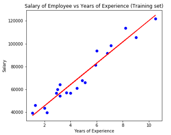
# Visualising the Test set results
Code:
plt.scatter(X_test, y_test, color = 'blue')

plt.plot(X_train, regressor.predict(X_train), color = 'red')

plt.title('Salary of Employee vs Experience (Test set)')

plt.xlabel('Years of Experience')

plt.ylabel('Salary')

plt.show()
# Parameter of model
Code:
print(regressor.intercept_)

print(regressor.coef_)

26816.19224403119

[9345.94244312]
So the interceptor (a) value is 26816. This suggests that any fresher (zero experience) would be getting around 26816 amount as salary.
The coefficient for our model came out as 9345.94. It suggests that keeping all the other parameters constant, the change in one unit of the independent variable (years of exp.) will yield a change of 9345 units in salary.
Regression Evaluation Metrics
There are basically 3 important evaluation metrics methods available for regression analysis:
- Mean Absolute Error (MAE): It shows the mean of the absolute errors, which is the difference between predicted and actual.
- Mean Squared Error (MSE): It shows the mean value of squared errors.
- Root Mean Squared Error (RMSE): It shows the square root of the mean of the squared errors.
We can compare the above methods:
- MAE: It shows the average error and the easiest of all three methods.
- MSE: This one is more popular than MAE because it enhances the larger errors, which in a result shows more insights.
- RMSE: This one is better than MSE because we can interpret the error in terms of y.
These 3 are nothing but the loss functions.
# Evaluation of model
Code:
from sklearn import metrics

print('MAE:', metrics.mean_absolute_error(y_test, y_pred))

print('MSE:', metrics.mean_squared_error(y_test, y_pred))

print('RMSE:', np.sqrt(metrics.mean_squared_error(y_test, y_pred)))

MAE: 3426.4269374307123

MSE: 21026037.329511296

RMSE: 4585.4157204675885
Conclusion
Linear Regression analysis is a powerful tool for machine learning algorithms used to predict continuous variables like salary, sales, performance, etc. Linear regression considers the linear relationship between independent and dependent variables. Simple linear regression has only one independent variable based on which the model predicts the target variable. We have discussed the model and application of linear regression with an example of predictive analysis to predict the salary of employees.
Recommended Articles
This is a guide to Simple Linear Regression. Here we discuss the introduction, what simple linear regression does, working, application & evaluation metrics. You can also go through our other related articles to learn more –