Updated August 22, 2023
Searching For Text in Excel
In this article, we will learn about Search For Text in Excel. you might have seen situations where you want to extract the text present at a specific position in an entire string using text formulae such as LEFT, RIGHT, MID, etc. You can also combine SEARCH and FIND functions to find the text substring from a given string. However, when you are not interested in finding out the substring but want to find out whether a particular string is present in a given cell, not all of these formulae will work. In this article, we will go through some of the formulae and/or functions in Excel, allowing you to check whether or not a particular string is present in a given cell.
How to Search Text in Excel?
Search For Text in Excel is very simple and easy. Let’s understand how to Search Text in Excel with some examples.
Example #1 – Using the Find Function
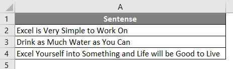
Let’s use the FIND function to find whether a specific string is present in a cell. Suppose you have data as shown below.
As we try to find whether a specific text is present in a given string, we have a function called FIND to deal with it on an initial level. This function returns a position of a substring in a text cell. Therefore, we can say that if the FIND function returns any numeric value, then the substring is present in the text; else, not.
Step 1: In cell B1, start typing =FIND; you can access the function itself.
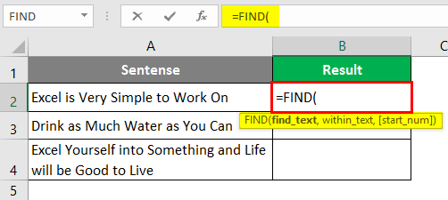
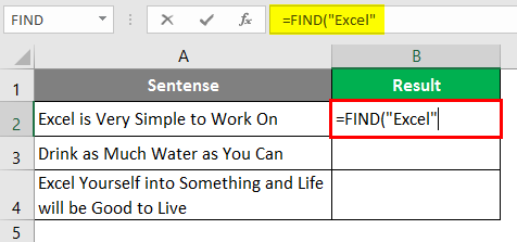
Step 2: The FIND function needs at least two arguments: the string you want to search and the cell within which you want to search. Let’s use “Excel” as the first argument for the FIND function, which specifies find_text from the formula.
Step 3: We want to find whether “Excel” is present in cell A2 under a given worksheet. Therefore, choose A2 as the next argument to the FIND function.
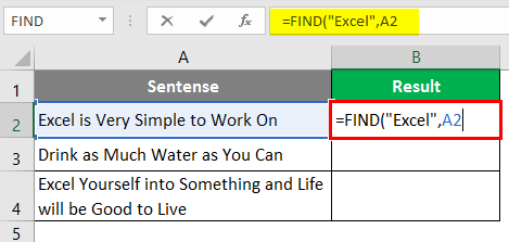
We are going to ignore the start_num argument as it is an optional argument.
Step 4: Close the parentheses to complete the formula and press Enter Key.
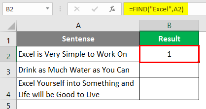
As you can see, this function returned the position where the word “Excel” is present in the current cell (i.e., cell A2).
Step 5: Drag the formula to see the position where Excel belongs under cells A3 and A4.
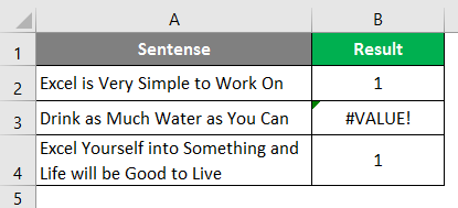
You can see in the screenshot above that the mentioned string is present in two cells (A2 and A3). In cell B3, the word is not present; hence, the formula provides the #VALUE! Error. This, however, doesn’t always provide a clearer picture. Someone might not be good enough to understand that 1 appearing in cell B2 is nothing but the position of the word “Excel” in the string occupied in cell A2.
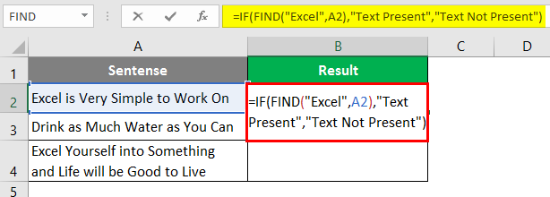
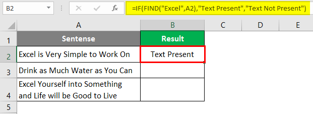
Step 6: To get a customized result under column B, use the IF function and apply FIND. Once you use FIND under IF as a condition, you must provide two possible outputs. One of the conditions is TRUE, and the other if the condition is FALSE. Press Enter after editing the formula with the IF condition.
After using the above formula, the output is shown below.
Step 7: Drag the formula from cell B2 to cell B4.
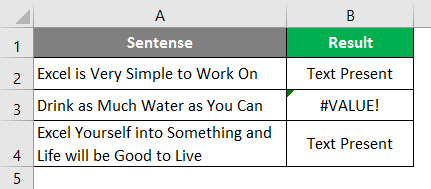
Now, we have used IF and FIND in combinations; the cell with no string still gives #VALUE! Error. Let’s try to remove this error with the help of the ISNUMBER function.
ISNUMBER function checks if the output is a number or not. When the output is a number, it will give TRUE as a value; if not a number, then it will give FALSE as a value. If we use this function in combination with IF and FIND, IF functions will give the output based on the values (either TRUE or FALSE) provided by the ISNUMBER function.
Step 8: Use ISNUMBER in the formula above in steps 6 and 7. Press Enter Key after editing the formula under cell B2.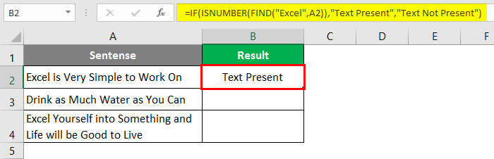
Step 9: Drag the formula across cell B2 to B4.
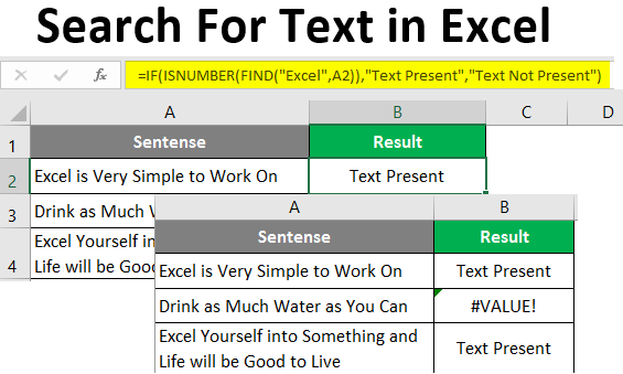
The #VALUE! error in previous steps was nullified due to the ISNUMBER function.
Example #2 – Using the SEARCH Function
Like the FIND function, the SEARCH function in Excel also allows you to search whether the given substring is present within a text. You can use it on the same lines; we have used the FIND function and its combination with IF and ISNUMBER.
The SEARCH function also searches the specific string inside the given text and returns the text’s position.
I will show you the final formula for finding if a string is present in Excel using the SEARCH, IF, and ISNUMBER functions. You can follow steps 1 to 9, all in the same sequence from the previous example. The only change will be to replace FIND with the SEARCH function.
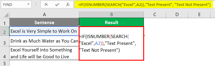
Use the following formula in cell B2 of the sheet “Example 2”, and press Enter Key to see the output (We have the same data as used in the previous example) =IF(ISNUMBER(SEARCH(“Excel”, A1)), “Text Present”, “Text Not Present”) Once you press Enter Key, you’ll see an output the same as in the previous example.
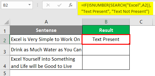
Drag the formula across cell B2 to B4 to see the final output.
In cells A2 and A4, the word “Excel” is present; hence it has output as “Text Present”. However, in cell A3, the word “Excel” is not present; therefore, it has output as “Text Not Present”.
This is from this article. Let’s wrap the things with some things to be remembered.
Things to Remember About Search For Text in Excel
- These functions check whether the given string is present in the text provided. If you need to extract the substring from any string, use the LEFT, RIGHT, and MID functions.
- ISNUMBER function is combined so that you are not getting any #VALUE! Error if the string is not present in the text provided.
Recommended Articles
This is a guide to Search For Text in Excel. Here we discuss How to Search Text in Excel, practical examples, and a downloadable Excel template. You can also go through our other suggested articles –
