Updated July 1, 2023
What is Power Query in Excel?
Power Query is a dynamic data connection tool designed for Excel. It allows users to import data from various sources, transform it to suit their needs and load it into their workbooks. Users can import data from Excel workbooks, CSV, XML, JSON, databases such as SQL Server, Access, Azure, and web pages.
The best part is that it comes with a query editor tool that remembers every change made to the data. This feature allows users to easily redo or edit any of the steps later by simply clicking the “refresh” button, automatically updating all the changes. With this tool, users don’t have to worry about repeating the same steps, making their job easier and more efficient.
How to Use Power Query in Excel?
Here’s a step-by-step guide on how to use Power Query:
Step 1. Open Excel and click on the “Data” tab in the ribbon.
Step 2. Click on the “Get Data” button and select your data source.
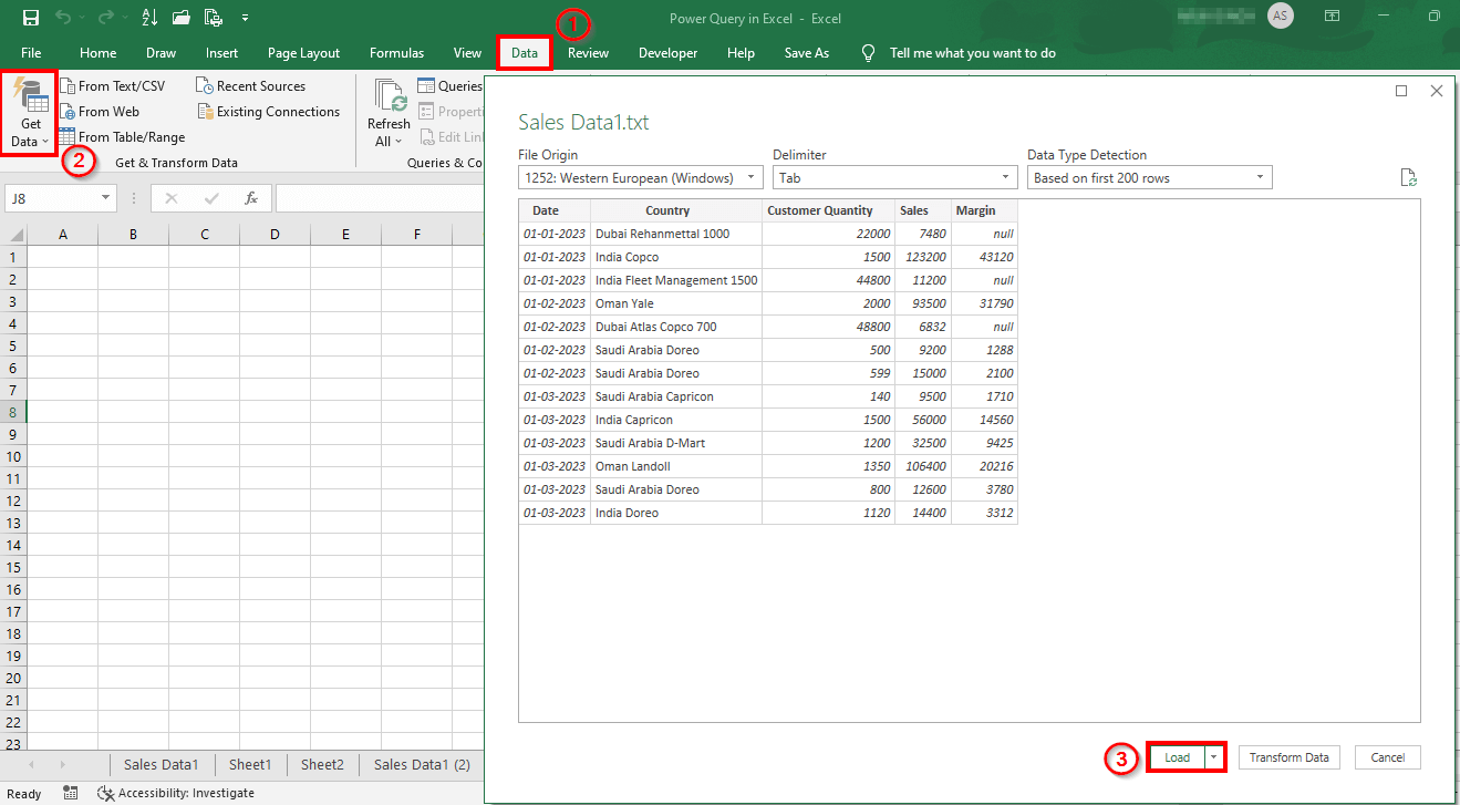
Step 3. Select the data you want to import and click the “Load” button.
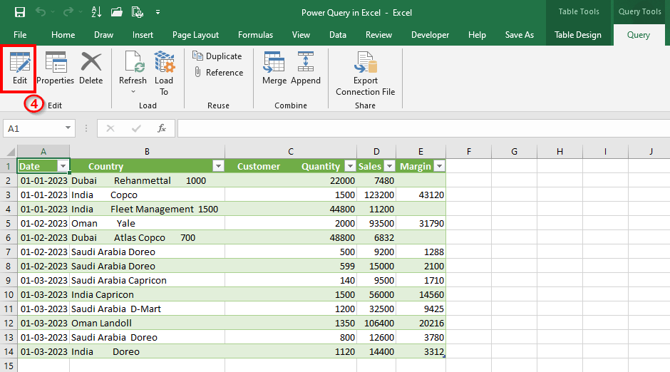
Step 4. Once the data is loaded, click the “Edit” button to open the Power Query Editor.
Step 5. In the Power Query Editor, you can perform various transformations on your data, such as filtering, sorting, and merging.
Step 6. To filter your data, click on the “Filter Rows” button. Now select the criteria you want to use.
Step 7. To sort your data, click the “Sort Ascending” or “Sort Descending” button.
Step 8. To merge data from different sources, click the “Merge Queries” button and select the tables you want to merge.
Step 9. Once you’re done with the transformations, click the “Close & Load” button to save your changes.
Example
Let’s take an example scenario where a text file contains 1000 rows of data stored in a folder. Now, let’s understand how to use the Power Query tool to easily import, edit, and add this data into an Excel worksheet.
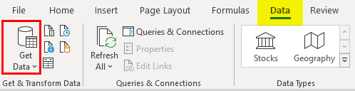
Step 1. Open a new Excel file and click the Data tab in the Excel ribbon
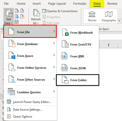
Step 2. Click the Get Data dropdown under the Get & Transform Data group.
Step 3. Click From File and then click From Folder.
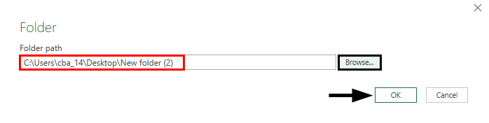
Step 4. Click Browse, navigate toward the path where you have the desired file, and click OK.
A new window shows a list of your saved files in the path.
Step 5. Select the desired file and click on Transform Data.

The window has four options at the bottom- Combine, Load, Transform Data, and Cancel.
- Combine- It allows you to combine or consolidate datasets from different sources having different file types. However, it has no separate Edit option, making it less versatile as you cannot decide which columns to combine.
- Load- It allows you to load the data as a table/Pivot into an Excel sheet, irrespective of the actual format of the data under the source file.
- Transform Data- It allows you to transform the data files irrespective of the source. You can also add a column with calculated values, change the format of specific columns, add or remove columns, group columns, etc.
- Cancel– It cancels or nullifies all other operations under the Power Query.
Click on the Transform Data tab. Once you click the Transform Data tab, the Power Query Editor window opens with the transformed data.
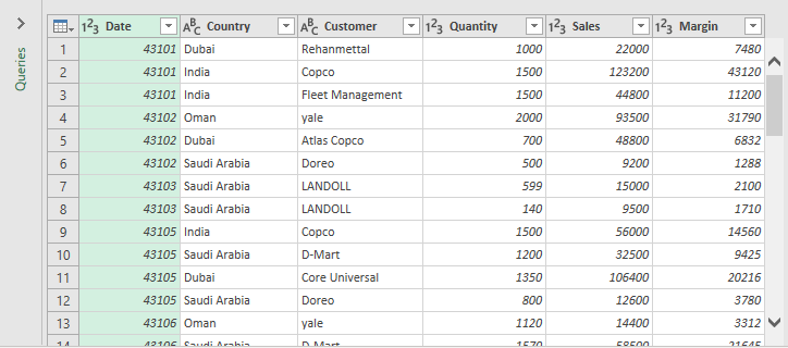
The Power Query Ribbon has five options- File, Home, Transform, Add Column, and View.
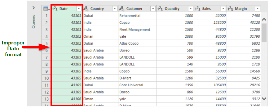
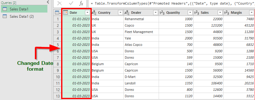
In the transformed data, the date is not in the proper format, as shown below.
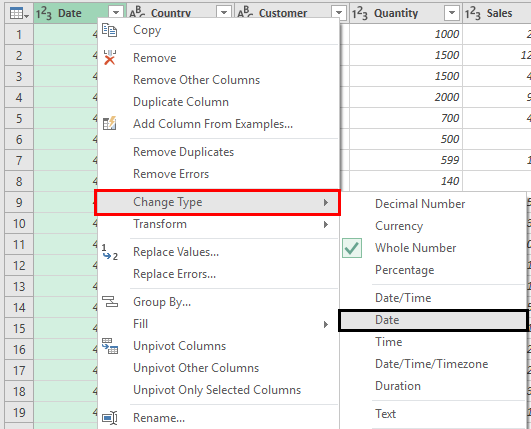
Step 6. To convert the date into the proper format, select and right-click on the Date column header, then select Change Type and click Date.
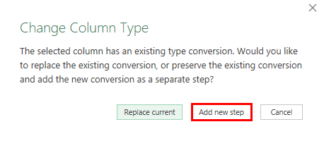
Step 7. A new window, Change Column Type, appears on the screen. Click Add a New step.
The values in the Date column have now changed to the proper format, as shown below.
We can add a column with computed/ calculated values to the existing data.
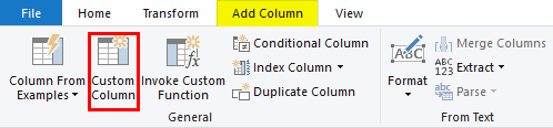
Step 8. Click Add Column > Custom Column under the General Group to add a new column to the data. It will allow you to create a new calculated column based on the custom formula.
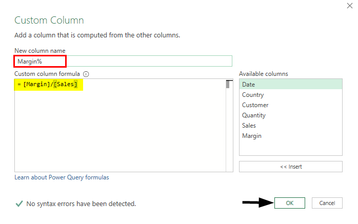
A Custom Column window appears on the screen. Here, we can give a name to the new column and enter a formula to provide calculated values.
We want to find the Margin in percentage; therefore, we will use the formula [Margin]/[Sales] and add the formulated values to a new column.
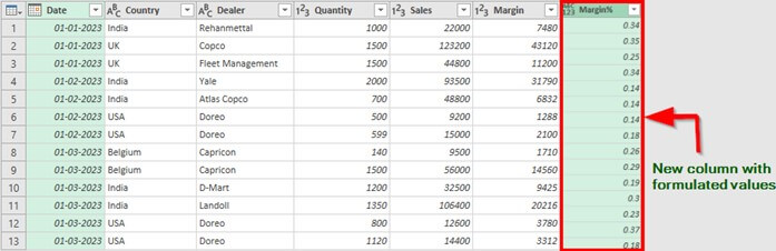
Step 9. To add the formulated data to the existing one, click the Add Column tab in the Editor Ribbon, enter the New column name as Margin%, the Custom column formula as [Margin]/[Sales], and click OK.
The Editor adds a new column to the data, as shown below.
We can work more on this data or prepare compelling reports by adding (loading) it into the Excel worksheet.
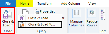
Step 10. To load the data into the Excel worksheet, go to Home in the Query Editor Ribbon
Step 11. Click Close & Load > Close & Load To…
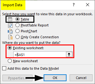
This option allows you to load the data as Table, PivotTable, PivotTable Chart, etc.
An Import Data wizard pops-up
Step 12. Select Table > Existing Worksheet or New Worksheet > OK.
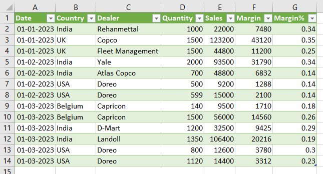
It loads the Sales Data in the existing worksheet/ new worksheet, as shown below.
Power Query Editor
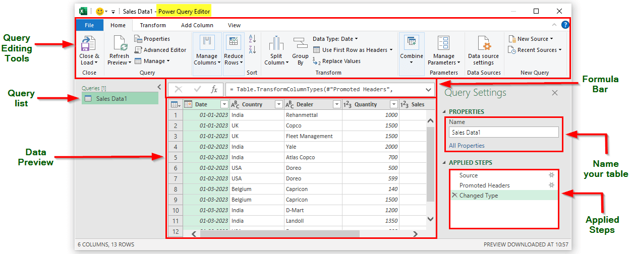
The Power Query in Excel consists of five sections- Query Editor Tools ribbon, Query Settings, Queries pane, Data Preview pane, and Formula Bar. Let’s understand them one by one:
- Query Editor Tools Ribbon– The Query Editor Ribbon has five tabs: File, Home, Transform, Add Column and View. The various data transformation options are available under these tabs.
- Queries –The Queries pane displays the lists of the Tables, Queries, and custom functions in an Excel workbook. It allows users to Duplicate, Rename or Navigate to different tables or queries in the current spreadsheet.
- Applied Steps/Query Settings – This pane chronologically lists each applied transformation step. When you select a specific step on this page, the Editor displays the result of the applied step in the Preview Grid. You can use this page to Rename, Reorder, or Delete transformation steps.
- Data Preview Pane – It displays the preview of imported data at each of the applied steps of a Query. The data preview pane provides different transformation options from the Column Header or by right-clicking on Individual cells.
- Formula Bar – Each applied transformation step of a Query has an M code (language used by Excel to write the corresponding code for each applied step in the Query Editor). The corresponding code is displayed in the Formula bar when you select a specific step from the Applied Steps pane. We can modify or edit the code using the Formula bar.
Query Editor Tools
The Power Query Editor tools are listed under the four tabs-
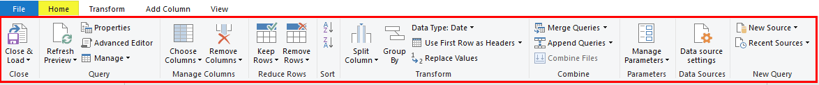
HOME- The HOME tab in the Power Query Editor Ribbon consists of the most commonly used options that allow users to edit/ delete queries, manage columns, reduce rows, sort data, and load it into Excel worksheets.
TRANSFORM- The options available in the TRANSFORM tab allow users to split existing columns, group data, change the data type, and replace values.

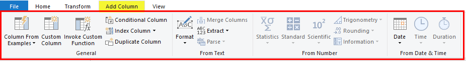
ADD COLUMN- Using the ADD COLUMN tab, users can add new custom columns, create index columns, duplicate columns, and create columns based on specific conditions.
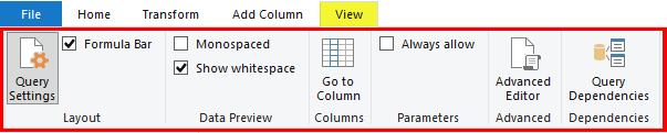
VIEW- The VIEW tab includes options to display/ hide the Formula bar, Query Settings/ Applied steps, Data Preview, and Columns.
When to Use Power Query in Excel?
Power Query is valuable in many scenarios where data needs consolidation, cleaning, transformation, or analysis. Here are some examples of when to use Power Query in Excel:
1. Consolidating Data from Multiple Sources
Power Query’s significant benefit is its ability to consolidate data from various sources into a single dataset.
For instance, a marketing team can use Power Query to pull data from various social media platforms, advertising networks, and email marketing tools to create a single dataset for analysis.
2. Cleaning and Transforming Data
Power Query includes various data cleaning and transformation features, making it easy to clean and prepare data for analysis.
For example, a financial analyst can use Power Query to clean and standardize financial data from multiple sources, eliminating errors and inconsistencies.
3. Automating Data Import and Analysis
Power Query automates importing and analyzing data, saving time and reducing errors.
For instance, a sales team can use Power Query to automatically import data from a CRM system and analyze trends and opportunities.
4. Merging Data from Different Formats
Power Query can merge data from various formats, such as CSV, Excel, and text files, into a single dataset.
For example, a supply chain analyst can use Power Query to merge data from different suppliers to identify potential bottlenecks and optimize the supply chain.
Best Practices
1. Give your queries intuitive and straightforward names before loading your data
- Define query names immediately. For instance, instead of naming your query “Query1”, give it a descriptive name such as “SalesData” or “CustomerRecords”. Updating table and query names later can be time-consuming and may lead to manual errors if you have referenced them in calculated measures.
- Avoid spaces in table names or enclose the space in double quotes.
2. Shape Data at the Source
- To minimize the need for complex steps, shape your data at the source (such as a database) before importing it into Excel. This approach allows you to create new data models without replicating the same procedure in the Query tool.
- For example, if you have a database with multiple tables, you can use SQL to join and filter the data before importing it into Power Query.
3. Load only the data you need when working with large tables
- Ensure you import only the data you need to load into Excel. Loading extra information may slow down the entire automation process unnecessarily.
Things to Remember
- The tool supports a maximum of 1,048,576 rows.
- You can build data models and create connections between tables.
- You can create a relationship between data tables based on common fields instead of linking them manually using formulas.
- Using Power Query, you can format text columns to a lower, upper, or proper case or add a prefix or suffix.
Frequently Asked Questions (FAQs)
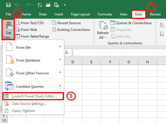
Q1. How do I enable Power Query in Excel?
Answer: To enable Power Query, follow these steps:
- Click the “Data” tab in the ribbon (at the top of the Excel worksheet).
- Select “Get Data“.
- Choose “Launch Power Query Editor” from the dropdown menu.
Q2. Is Power Query available in all Excel?
Answer: Power Query is available in all stand-alone Windows versions of Excel 2016 or later, as well as with subscription plans of Microsoft 365. In the case of earlier Excel versions, users can install the Power Query Editor as an add-in.
Q3. Why can’t I see Power Query in Excel Mac?
Certain license types do not include Power Query in Excel for Mac. Additionally, some business license types may only receive the new Power Query features once or twice a year. The IT and education departments may control licenses that do not have the feature until the respective administrators roll it out.
Q4. What is the difference between Excel Power Query and Power Pivot?
Answer: Here’s a table that summarizes the differences between Power Query and Power Pivot:
|
Difference |
Power Query |
Power Pivot |
| Function | Imports and transforms data from multiple sources for analysis | Analyzes and models data to produce insights |
| Main task | Prepares and cleans data for analysis | Analyzes data to produce insights |
| Data sources | Excel files, CSVs, databases, websites, and more | Excel workbooks or data models |
| Data transformation | Combines, filters, sorts, and cleans data | Creates calculated columns, measures, and relationships between data |
| Visualization | No built-in visualization capabilities | Offers data visualization tools like charts and pivot tables |
| Skill level required | Beginner to intermediate Excel users | Intermediate to advanced Excel users |
Recommended Articles
The above article is a guide to Power Query in Excel. Here we discuss using Power Query and importing data from different databases with examples. You can also go through our other suggested articles-