


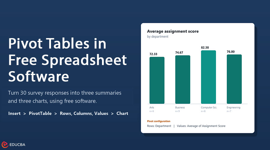
Thirty survey responses and eight columns look manageable until the question is average score by department, students per study method, and hours by year. Pivot Tables in free Spreadsheet software make these tasks easier by summarising data without complex formulas. A pivot table organizes information into meaningful categories, while charts turn the results into clear visual comparisons.
This step-by-step guide uses WPS Spreadsheets and a sample dataset of 30 student responses. It explains how to create pivot tables, generate charts, interpret results, and fix common errors.
What a Pivot Table Does?
A pivot table summarises a larger table. You choose which columns become row labels, which become column labels, and how the numbers are calculated. The source rows stay untouched.
Four areas control it: Rows group records down the page, Columns across, Values hold the numbers, and Filters restrict the table to one category. Move a field and the same data is summarised differently, which is where the name comes from.
For other layouts, the EDUCBA collection of pivot table examples covers common configurations.
Why Use Pivot Tables in Free Spreadsheet Software for Course Assignments?
The academic questions are narrow: average marks by department or year, counts per survey option, and a data-quality check, because a count per category exposes blanks and misspellings faster than scrolling. Each is comparative, and a pivot answers one in about the time it takes to drag two fields.
Set Up the Data First
Three rules prevent most of the problems below:
- One header row, with a name in every column.
- One record per row: no subtotals, no spacer rows, no merged cells.
- Real numbers in numeric columns, because a score stored as text is counted, not averaged.
Build the First Pivot Tables in Free Spreadsheet Software
WPS Spreadsheets provides a straightforward way to create pivot tables. Follow these steps:
- Click any cell in the range, then Insert > PivotTable.
- Confirm the source reads A1:H31, then choose New worksheet so the raw data stays intact.
- Drag Department into ROWS, then Assignment Score into VALUES. WPS adds it as Sum by default.
- Right-click a value, open Summarize Values By, and choose Average.
Read the count in the corner: if it is not 30, the range is wrong. After editing the source, right-click the pivot and refresh; if you added rows, use Change Data Source.
WPS is used because its pivot workflow matches Excel. Students weighing a free Microsoft Office alternative should check how the free version handles submitted files; this overview of free spreadsheet software covers the rest.
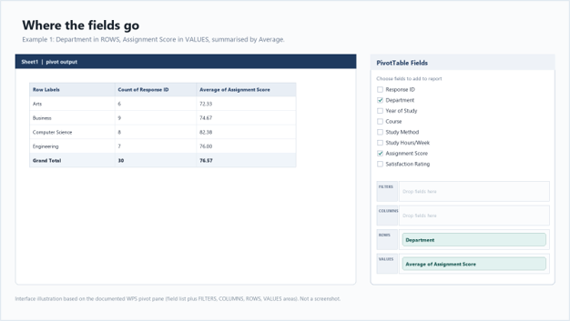
Figure 1: Department in ROWS, average score in VALUES.
Three Examples That Cover Most Assignments
The following examples demonstrate how pivot tables can answer common academic questions. Each summary uses the same dataset of 30 student responses.
Example 1: Average Score by Department
Rows: Department. Values: Average of Assignment Score. Columns and Filters stay empty.
| Department | Students | Average score |
| Arts | 6 | 72.33 |
| Business | 9 | 74.67 |
| Computer Science | 8 | 82.38 |
| Engineering | 7 | 76.00 |
| Grand total | 30 | 76.57 |
Computer Science leads at 82.38, about 5.8 points above the overall 76.57, and Arts trails at 72.33. Report group sizes with the averages: Arts has six students and Engineering seven, so one unusual score moves those means further.
Example 2: Students by Study Method
Rows: Study Method. Values: Count of Response ID, because counting an ID counts records.
| Study Method | Students | Share of 30 |
| Self-Study | 11 | 36.7% |
| Group Study | 8 | 26.7% |
| Online Videos | 6 | 20.0% |
| Tutoring | 5 | 16.7% |
| Total | 30 | 100.0% |
Self-Study is the most common method at 11 of 30, and the gap to Group Study is three students, small enough that another sample could reverse it. Write in this sample rather than what most students prefer.
Example 3: Average Hours by Year
Rows: Year of Study. Values: Average of Study Hours per Week.
| Year of Study | Students | Average Hours Per Week |
| First Year | 8 | 9.75 |
| Second Year | 8 | 12.88 |
| Third Year | 8 | 17.00 |
| Fourth Year | 6 | 18.50 |
| Grand total | 30 | 14.27 |
Hours rise every year, from 9.75 to 18.50, with the largest step between the second and third, and the fourth-year mean is the least stable because that group is smallest.
Turn Each Summary into a Chart
Chart the summary, not the raw rows, and leave the grand total out or it flattens the comparison.
- Select the category and value columns from the summary, including the header row.
- Insert > Chart > Column > Clustered Column.
- Title it Average assignment score by department, label the vertical axis Average score (out of 100), and keep labels horizontal.
Bar charts suit the longer study-method labels, and columns suit the four-year groups, so the gaps between them stay visible.
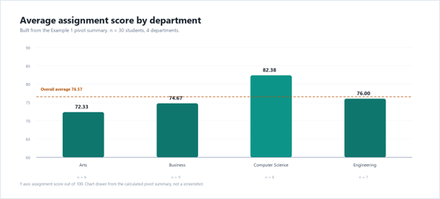
Figure 2: the Example 1 summary as a column chart.
EDUCBA’s guide to the pivot chart covers the other chart types.
Read the Results Before You Write
A table is evidence; the marks sit in the paragraph that says what it means.
“Average weekly study hours rise with year of study, from 9.75 in first year to 18.50 in fourth (Table 3). The largest step is between second and third year, 4.13 hours. Fourth-year students report the highest average but form the smallest group (n = 6), so their mean is the least stable. These figures describe the 30 responses collected, not the wider population.”
Attribute every number to a table, avoid causal verbs the design cannot support, and state sample sizes when comparing groups.
For formula-based work, EDUCBA’s overview of the data analysis tool in Excel is a useful companion.
Fix the Usual Problems
| Symptom | Likely Cause | Fix in WPS Spreadsheets |
| Average comes back as a sum | Sum is the default aggregation | Right-click the value, Summarize Values By, Average |
| Count is lower than the rows | Blank rows, or blank cells in the grouped column | Delete or fill the blanks, then Refresh |
| Scores average to 0 | Numbers stored as text | Convert the column to numbers, then Refresh |
| New rows are ignored | Refresh keeps the original range | Analyze > Change Data Source, select the larger range |
Two are worth memorizing: text numbers break averages silently, and a stale range makes a correct pivot look wrong.
Final Thoughts
Pivot Tables in free Spreadsheet software help students organize, summarise, and analyze academic data without complicated formulas. They make it easier to compare departmental scores, count survey responses, and identify changes in study habits.
Keep an untouched copy of the file and build pivots on a duplicate. Name fields the way you would say them aloud. Submit a format that keeps your layout, because a PDF preserves chart placement and a re-typed table does not. Open the file on a phone before submitting, which any free document reader will do.
A pivot table asks a comparative question without formulas, and a chart is the same answer in a form a reader absorbs in seconds. Rebuild the three examples and compare your counts with the tables above.
Recommended Articles
This comprehensive guide to Pivot Tables in Free Spreadsheet Software helps simplify data analysis and improve academic assignments. Check out these recommended articles for more insights and practical tips on spreadsheet tools, data organization, and data visualization.