Updated May 8, 2023
NPER Function in Excel (Table of Contents)
Introduction to NPER Function in Excel
NPER stands for the Number of Periods. NPER means the number of periods to pay back the loan. The NPER function is one of the in-built financial functions in MS Excel. It helps calculate the period required to pay back the total loan amount periodically at a fixed interest rate.
Syntax of NPER Function:
Arguments of NPER Function:
- Rate:- It is the rate of interest per period.
- Pmt:- It is the installment payment, done yearly or monthly as applicable. It includes only a principal amount and interest. No other charges are included.
- Pv:- It is the present value for future payments.
- fv:– It is the future value of the cash we want after the tenure, i.e., after the last payment. It is optional, hence can be taken as zero or omitted.
- Type:- It indicates when a payment is due. It is optional. The “Type” parameter can have the following values:
- If the Type is taken as 0 or omitted, payments are due at the end of the project.
- If the Type is taken as 1, it means payments are due at the project’s start.
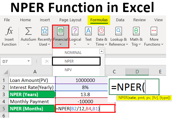
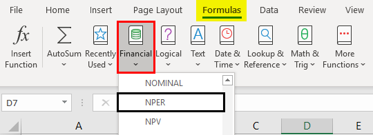
Go to the Formulas tab in Excel Ribbon-> Click on Financial dropdown list-> select “NPER.”
Examples of NPER Function in Excel
The following examples demonstrate how to calculate NPER. Assume PMT and Rate remain constant throughout the tenure.
Example #1 – NPER Function (FV and Type are Omitted)
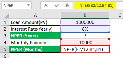
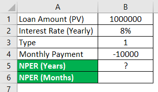
Ms. ABC took a loan of Rs.1000000 at an interest rate of 8% per annum. She can pay a monthly EMI amount of Rs.10000. Does she want to determine the months to repay her loan?
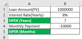
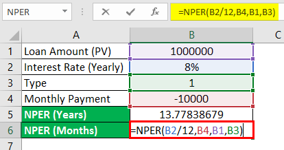
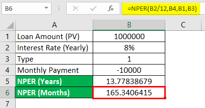
I am using NPER Function in cell B5.
After using the function, the answer is shown below.
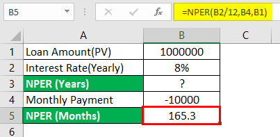
In the above example, the yearly rate, i.e., “Interest Rate (Yearly)”, is converted monthly, i.e., B2/12, and used as a first argument. The next input, Pmt, “Monthly payment,” goes as a second argument, i.e., B4. Here, PMT is marked negative to show an outgoing amount. “Loan Amount (PV)” goes as a third argument, i.e., B1. In this example, Fv and type are omitted since those are optional.
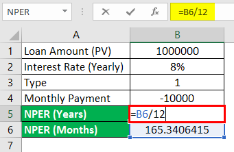
To convert the “NPER (Months)” into Years.
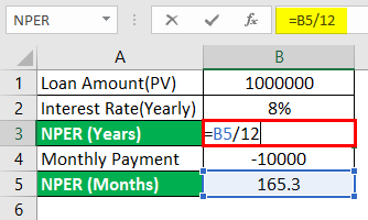
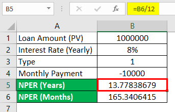
After converting the “NPER (Months)” in Years, the answer is shown below.
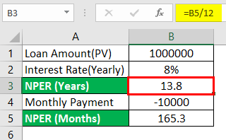
Therefore, Ms. ABC, by paying a monthly EMI of Rs.10000, can clear the loan in 13 years and 8 months.
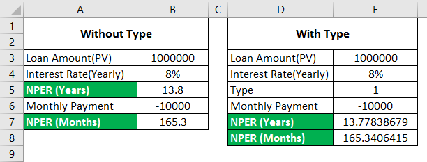
Example #2 – NPER Function (Type is 1 and Fv is Omitted)
In the example above, we will use Type to get periods in month and year.
To convert the “NPER (Months)” into Years.
After converting “NPER (Months)” to Years, the answer is shown below.
Everything is the same as above. The only Type is taken as 1 instead of omitting the same.
After using Function, the answer is shown below.
A difference is observed in the value calculated for NPER (Months) or NPER (Years) based on the Type.
- If the Type is set to 0 or omitted, payments are due at the end of the period.
- If the Type is set to 1, payments are due at the start of the period.
Example #3 – NPER Function with FV and Type is 0
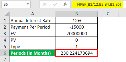
Ms. ABC is doing financial planning for her retirement. She plans to make an amount of Rs.2,00,00,000 by investing Rs.15000 per month at a fixed interest rate of 15% p.a. Calculate the number of periods that she needs to make an amount of Rs.2,00,00,000.
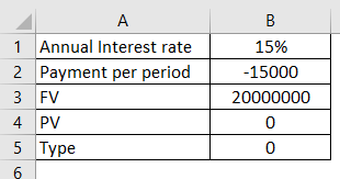
We are using NPER Function in cell B6 with Type 0.
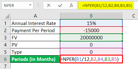
After using the function, the answer is shown below.
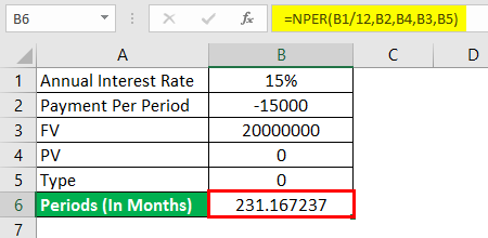
In the above example, the yearly rate, i.e., “Interest Rate (yearly)”, is the input that is converted every month (B1/12) and used as a first argument. The next input is Pmt, the monthly payment (B2), used as a second argument. Here, Pmt is marked as negative to show an outgoing amount. Since the loan is not involved here, PV (B4) is taken as 0 and used as a third argument. Here, FV (B3) is being taken as the third argument, and Type may be taken as 0 or omitted, being optional.
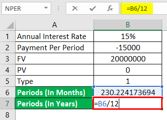
To convert “NPER(Months)” into “NPER(Years).”

After converting “NPER(Months)” into “NPER(Years)”, the answer is shown below.
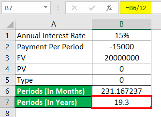
Hence, by paying a monthly amount of Rs.15000, Ms. ABC can make Rs.2,00,00,000 in 19 years and 3 months (approx.).
Example #4 – NPER Function with FV and Type is 1
Taking the above example, we will use Type 1 to get periods in months and years.
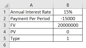
We are using NPER Function in cell B6 with Type 1.
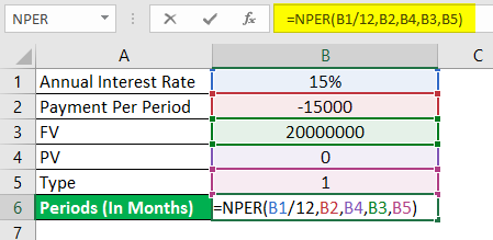
After using the function, the answer is shown below.
To convert “NPER(Years)” into “NPER(Months).”
After converting periods (In Years), the answer is shown below.

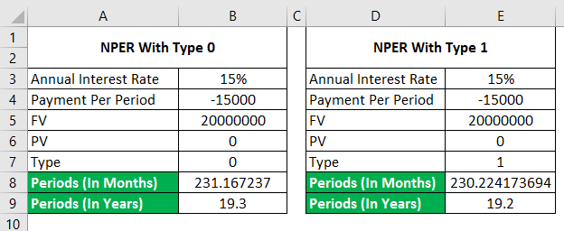
Hence, by paying a monthly amount of Rs.15000, Ms. ABC can make Rs.2,00,00,000 in 19 years and 2 months (approx.).
The difference in Ex 3 and Ex 4 is observed because of Type.
Things to Remember About NPER Function in Excel
- Per the cash flow convention, outgoing payments are marked as negative and incoming cash flows as positive.
- The currency, by default, is the dollar ($). This can be changed as per the following –
- Fv and Type are optional.
- Payment and rate are adjusted for monthly, quarterly, half-yearly, annually, etc.
- Always use the “=” sign for writing the formula in the active cell.
Recommended Articles
This is a guide to NPER Function in Excel. Here we discuss How to use NPER Function in Excel, practical examples, and a downloadable Excel template. You can also go through our other suggested articles –
