Table of Contents
- What is a Matrix In Excel?
- How to Create a Matrix in Excel?
- Calculations on Matrix in Excel
- Transpose of Matrix in Excel
- How to Inverse a Matrix in Excel?
- Find the Determinant of Matrix in Excel
What is a Matrix in Excel?
A Matrix is an arrangement of data (numbers or equations) in rows and columns that looks like a rectangular or square. It is an important data visualization tool in mathematics that helps solve mathematical linear equations.
- It is represented by mxn (m multiplied by n), where m is the number of rows and n is the number of columns.
- The most common matrix is the 3×3 matrix, which has 3 rows (m) and 3 columns (n).
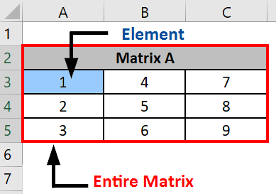
- Each data added to a matrix is called an element of the matrix.
- When you multiply the m and n, i.e., the rows and columns of a matrix, you get the total number of elements present in a matrix.
Creating a matrix in Excel can help mathematicians, students, and other professionals easily perform complex matrix calculations using Excel formulas and functions.
Here’s an example of a 3×3 matrix with 9 elements:
How to Create a Matrix in Excel?
Follow these steps to create a matrix in Excel:
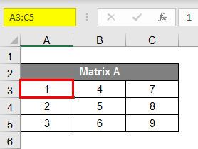
- Create a table with the number of rows and columns you want in the matrix. E.g., 3×3.
- Fill the data in the cells.
- Add a name (heading) to the matrix. Every matrix should have a unique name. For instance, we have named the below matrix: Matrix A.
Calculation on Matrix in Excel
Let us see how we can perform calculations like addition, subtraction, and multiplication on matrices in Excel.
1. Addition
Adding two matrices is similar to adding numbers in two rows or columns.
Steps:
⇒ First, make sure that both matrices have the same number of rows and columns.
⇒ Create a new third matrix that has the same number of rows and columns as the matrices you want to add.
⇒ In the first element of the new matrix, add the first elements of the two matrices together.
⇒ Drag the formula to other elements of the matrix.
Example:
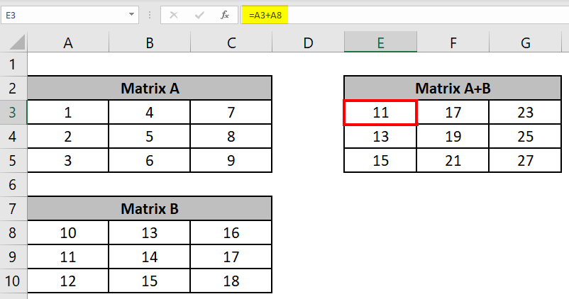
Suppose we have two matrices: A & B. Here, we add the formula =A3+A8 in the 1st element of the third matrix. It adds both 1st elements of matrix A & B.
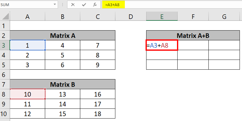
Now, drag the formula till columns E and G to apply the formula to all elements of the third matrix. Now, you can see the addition of these cells shown in the new matrix.
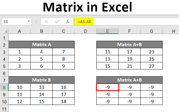
2. Subtraction
Similar to addition, subtracting two matrices is like subtracting numbers present in two columns.
Steps:
⇒ Ensure that the number of rows and columns in both matrices is the same, and create a new matrix with the same number of rows and columns.
⇒ In the first element of the third matrix, subtract the first element of the second matrix from the first element of the first matrix.
Example:
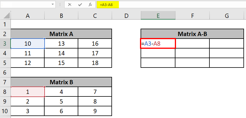
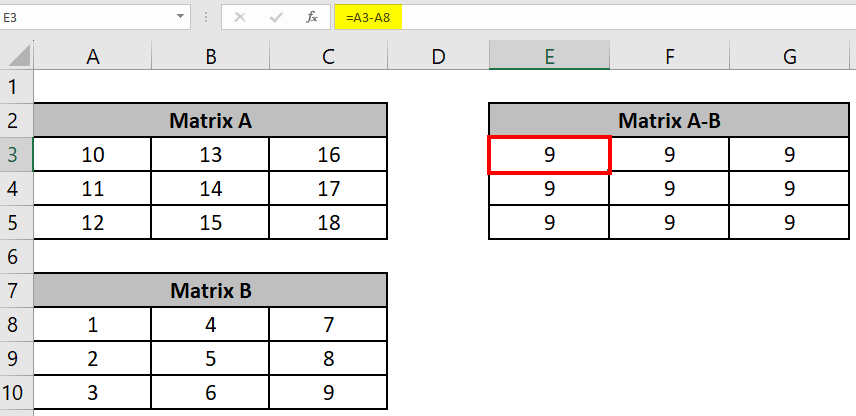
Let’s say you have two matrices: A & B. Here, first, we use the formula =A3-A8 in the 1st element of the third matrix. It subtracts both 1st elements of matrix A & B.
Similarly, subtract the formulas for all elements, and you can see the subtracted values in the third matrix.
3. Multiplication
Multiplication of matrices is not as simple as addition and subtraction. However, Excel makes it easier to multiply two matrices using the MMULT() function. So, let us see how to multiply the matrix in Excel.
Example:
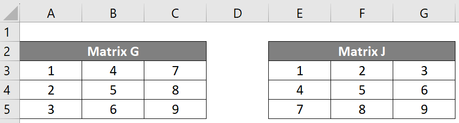
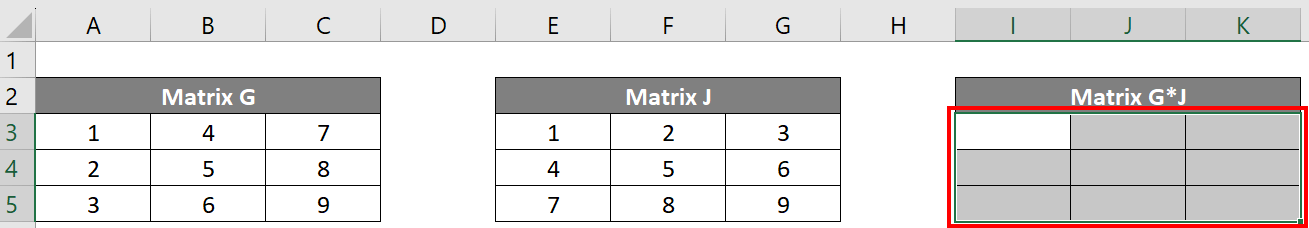
Let’s take two different 3X3 matrices: Matrix G and Matrix J.
Step 1: Create a new matrix with the same number of rows and columns.
Step 2: Select the range of the new matrix, e.g., I3: K5.
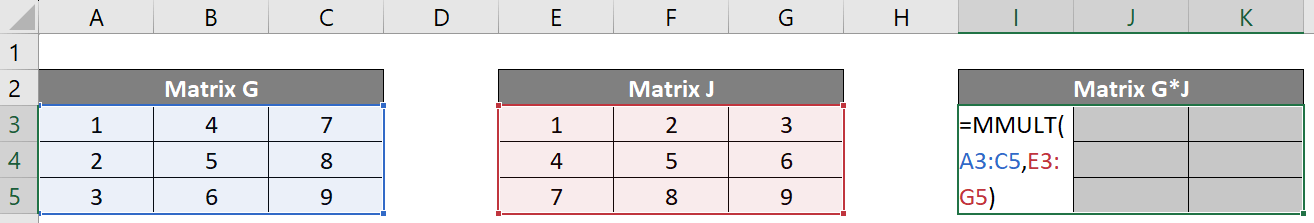
Step 3: Type the formula =MMULT(A3:C5,E3:G5) where A3:C5,E3:G5 is the range of your first and second matrices.
Step 4: Press Ctrl+Shift+Enter.
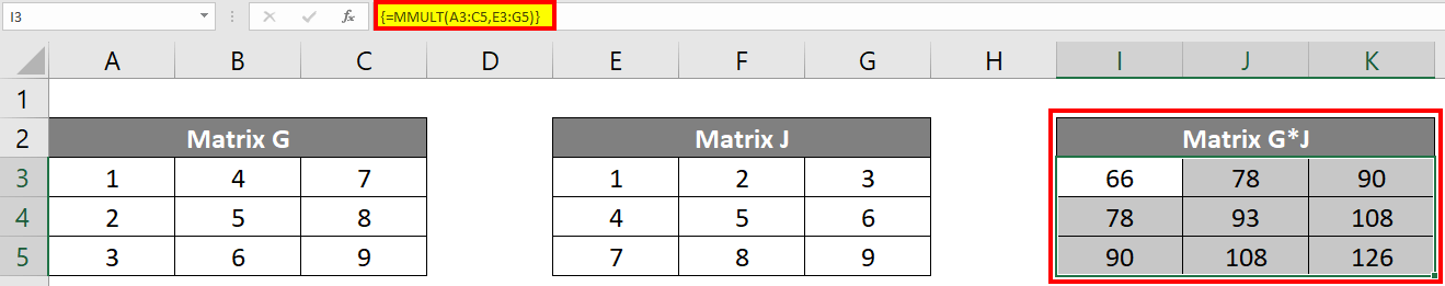
Result:
The third matrix shows the multiplication of Matrix G and J elements.
Transpose of Matrix in Excel
Transpose of a matrix involves flipping a matrix where the resulting matrix has the same elements, but they are reorganized differently. It means the row elements become column elements, and the column elements become row elements. If you have a matrix I, the transpose of I is usually denoted as I^T.
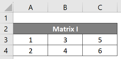
Example:
Let’s say you have a matrix I with dimensions 2 x 3, which means it has 2 rows and 3 columns.
Steps:
- Create a new matrix with nxm dimensions. It means the number of rows becomes the number of columns, and vice versa.
- Select the range of the new matrix, e.g., E3: F5.
- Type the formula =TRANSPOSE(A3:C4), where A3:C4 is the range of Matrix I.
- Press Ctrl+Shift+Enter.
Result:
How to Inverse a Matrix in Excel?
An inverse matrix is also known as a multiplicative inverse or reciprocal matrix. It is a matrix that you get when you multiply a matrix with an identity matrix. In Excel, you can easily find the inverse of a matrix by using the MINVERSE() function.
Example:
Suppose you have a 3×3 matrix E.

Steps:
⇒Select the range (Eg., E3:G5) where you want the inverse matrix to appear.
⇒Enter the following formula as an array formula: =MINVERSE(A3:C5), where A3:C5 is the range of matrix E.
⇒Press Ctrl+Shift+Enter.
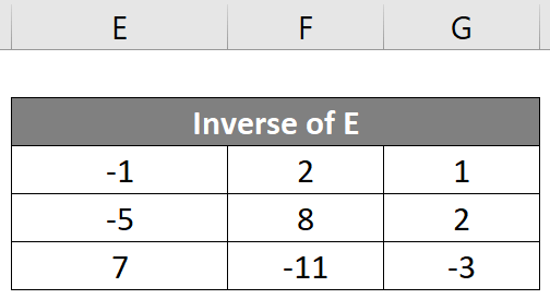
Result:
You will have an inverse of matrix E.
Note:
- The matrix must be square, with the same number of rows and columns.
- If there are empty cells in the matrix, MINVERSE won’t work, showing an error (#VALUE!).
- If the matrix doesn’t meet the square rule (equal rows and columns), it will show an error (#VALUE!).
- Sometimes, some matrices can’t be inverted; hence, MINVERSE will show an error (#NUM!).
Determinant of Square Matrix in Excel
The determinant of a square matrix is a single number that tells us about the scaling property of the matrix. To find the determinant of a matrix in Excel, you can use the MDETERM() function. This method is suitable for relatively small matrices and provides a straightforward way to find the determinant in Excel.
Example:
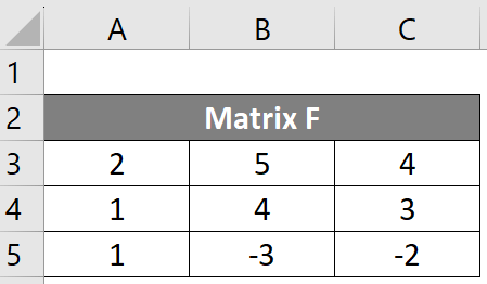
Imagine we have the below matrix F.
Solution:
In an empty cell where you want to display the determinant, input this formula: =MDETERM(A3:C5), where A3:C5 is the range of the Matrix F.
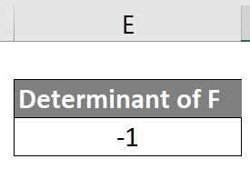
Result:
The determinant of Matrix F is -1.
Note:
- The matrix must be square, meaning it has the same number of rows and columns. Thus, if the matrix doesn’t meet the square rule (equal rows and columns), it will also show an error (#VALUE!).
- If there are empty cells or text in the matrix, MDETERM won’t work, and it will show an error (#VALUE!).
Recommended Articles
This article guides you on how to create a Matrix in Excel. You may also look at these useful functions in Excel,
