Updated March 4, 2023
Introduction of Matlab polyfit()
MATLAB function polyfit() is defined to fit a specific set of data points to a polynomialquickly and easily computing polynomial with the least squares for the given set of data. It generates the coefficients for the elements of the polynomial, which are used for modeling a curve to fit to the given data.
Polyfit() function uses input vector (x) to form Vandermonde matrix (V ) having n+1 columns and r = length(x) rows, which is nothing but results in a linear system.
Syntax of Matlab polyfit()
Syntax of Matlab polyfit() are given below:
|
Syntax |
Description |
poly = polyfit(x,y,n) |
It generates the coefficients of the resultant polynomial p(x) with a degree of ‘n’, for the data set in yas the best fit in the view of a least-square. The coefficients in p are assigned to power in descending order and matching length of p to n+1. |
[poly,Struct] = polyfit(x,y,n) |
It results in a structure S which can be used as input to the function polyval() in order to obtain error estimation. |
[poly,Struct,mu] = polyfit(x,y,n) |
It results in a two-element vector having values-centered and scaled.
mu(1) holds a value of the mean of (x), and mu(2) ) holds the value of standard of (x). Using these two values, function polyfit()makes x centered at zero and scaledx to have a unit standard deviation,
|
Input Arguments
- Query Points: Query points are specified as an input of vector type. If x is non-vector element, then this function polyfit() converts x into a column vector.The data points in x and their corresponding fitted function values contained in the vector y are formed.
Note
If the vector x has recurring data points or if it needs centering and scaling, warning messages may result out.
- Fitted values at query points: Fitted values as inputs are available at query points being specified with the vector data type. The data points in x and their corresponding fitted function values contained in the vector y are formed. If y is the non-vector element, then this function polyfit() converts y into a column vector.
- Degree of polynomial fit: Degree of polynomial fit as inputs, are available being specified as any positive integer scalar. In the respective syntax, ‘n’refers to the polynomial power to that of the left-most coefficient in the polynomial ‘p’.
Example of Matlab polyfit()
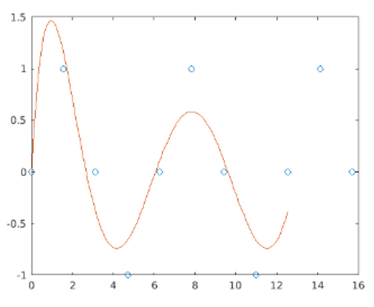
The below code is designed to generate data points placed equally spaced across a sine curve drawn in a specific interval.
Code:
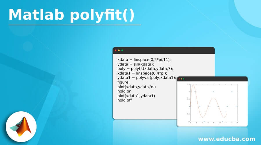
xdata = linspace(0,5*pi,11);

ydata = sin(xdata);

poly = polyfit(xdata,ydata,7);

xdata1 = linspace(0,4*pi);

ydata1 = polyval(poly,xdata1);

figure

plot(xdata,ydata,'o')

hold on

plot(xdata1,ydata1)

hold off
Output:
Use Cases for polyfit() Function
Use cases for polyfit() function are given below:
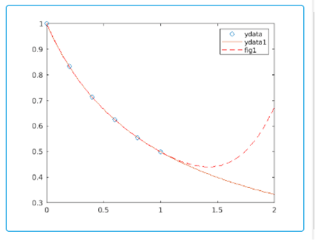
Fitting Polynomial to Set of data Points: The below code snippet carry out the fitting process on the polynomial poly of degree 4 towards 5 points.
Code:
xdata = linspace(0,1,6);

ydata = 1./(1+xdata);

poly = polyfit(xdata,ydata,4);

xdata1 = linspace(0,2);

ydata1 = 1./(1+xdata1);

fig1 = polyval(poly,xdata1);

figure

plot(xdata,ydata,'o')

hold on

plot(xdata1,ydata1)

plot(xdata1,fig1,'r--')

legend('ydata','ydata1','fig1')
Output:
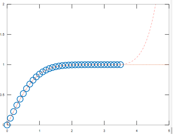
Fitting the Polynomial function to Error Function: The below code generate a vector having x data points being placed equally in the interval of [0,3.5] and co-efficient are assigned to the polynomial assuming the degree as 6.
Code:
xdata = (0:0.1:3.5)';

ydata = erf(xdata);

poly = polyfit(xdata,ydata,6)

func = polyval(poly,xdata);

T = table(xdata,ydata,func,ydata-func,'VariableNames',{'X','Y','Fit','FitError'})

xdata1 = (0:0.1:5)';

ydata1 = erf(xdata1);

func1 = polyval(poly,xdata1);

figure

plot(xdata,ydata,'o')

hold on

plot(xdata1,ydata1,'-')

plot(xdata1,func1,'r--')

axis([0  5  0  2])

hold off
Output:
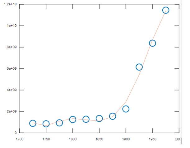
Improving Numerical Properties using Centering and Scaling: While solving the equation p = V\y, the condition number for V is usually large for higher-order fits and results in a matrix with singular coefficient, as the columns of V (Vandermonde matrix) are powers of the x vector.
In such cases, functions like scaling and centering are helpful to improve the numerical properties associated with the system in order to find a fit that is more reliable. In the below example polyfit() is called on three outputs to fit a polynomial of degree 5 along with the process of centering and scaling. The data is centered for the quarter, at 0, and scaled to have a unit standard deviation.
Code:
quarter = (1725:25:1975)';

data = 1e6*[891 846 938 1250 1272 1344 1550 2232 6142 8370 11450]';

Tab = table(quarter, data)

plot(quarter,data,'o')

[poly,~,mu] = polyfit(Tab.quarter, Tab.data, 5);

func = polyval(poly,quarter,[],mu);

hold on

plot(quarter,func)

hold off
Output:
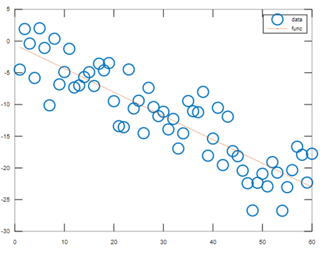
Simple Linear Regression: A simple linear regression model can be used to apply a fitting to a set of discrete two-dimensional data points.
Code:
xdata = 1:60;

ydata = -0.4*xdata + 3*randn(1,60);

poly = polyfit(xdata,ydata,1);

xdata = 1:60;

ydata = -0.4*xdata + 3*randn(1,60);

poly = polyfit(xdata,ydata,1);

func = polyval(poly,xdata);

plot(xdata,ydata,'o',xdata,func,'-')

legend('data','func')
Output:
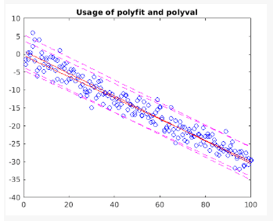
Combining Linear Regression and Error Estimation: A linear model can be set fit to a set of specified data points and the results can be plotted including an estimation of a prediction interval of 95%.
A few vectors can be created containing sample data points. The function polyfit can be called to fit a polynomial of degree 1 to the given set of data. Dual outputs can be specified to hold the values of coefficients supporting a linear fit as well as a structure containing error estimation.
Code:
xdata = 1:100;

ydata = -0.3*xdata + 2*randn(1,100);

[poly,Samp] = polyfit(xdata,ydata,1);
/*The error estimation structure is specified as the third input so that the function polyval()computes an estimated standard error. The estimated standard error estimate is stored in the second output variable delta. */
[yaxis_fit,delta] = polyval(poly,xdata,Samp);

plot(xdata,ydata,'bo')

hold on

plot(xdata,yaxis_fit,'r-')

plot(xdata,yaxis_fit+2*delta,'m--',xdata,yaxis_fit-2*delta,'m--')

title('Usage of polyfit and polyval')
Output:
Additional Note
- For n number of data points, a polynomial can be fit to that of degree n-1 to passing exactly through the points.
- With the increase in the degree of the polynomial, a fitting process using polyfit()loses the accuracy resulting in to a poorer fit for the data. In such cases, a low-order polynomial is preferable to use that tends to be smoother between the data points or apply a different technique, based on the requirement.
- This process of transformation using scaling and centering, add an advantage to the numerical properties of both the polynomial as well as to the fitting algorithm.
Recommended Articles
This is a guide to Matlab polyfit(). Here we also discuss the introduction and use cases for polyfit() function along with examples and its code implementation. you may also have a look at the following articles to learn more –
