Updated March 4, 2023

Introduction to MATLAB Plot legend
MATLAB provides plenty of functionalities useful in various computational problems. As we learned in previous articles, we can create vector plots in MATLAB using the ‘plot’ function. This article will teach us how to put Legends into the plots created in MATLAB. First, let us understand why we need to have legends for our plots. We create plots to visualize our data, and as we learned already, a single plot can have more than 1 vector or function. In such cases, we must provide more info about the functions drawn in the plot Legends are the way to provide information about different functions contained in a single plot In this topic, we are going to learn about Matlab Plot Legend.
Syntax
The syntax for creating Legends in MATLAB:
legend

legend(L1, L2, ...., L N) , where L1, L2 and so on represents the respective labels.
Explanation: This function will create a legend for each data series used in the plot, with descriptive labels. The function ‘legend’ will create labels like ‘data1’, ‘data2’, and so on.
Table for direction codes
| Direction | Code |
| Top of the axes | north |
| Bottom of the axes | south |
| Right of the axes | east |
| Left of the axes | west |
| Top right the axes | northeast |
| Top left of the axes | northwest |
| Bottom right | southeast |
| Bottom left | southwest |
Examples to Implement Matlab Plot Legend
Let us understand the function with an example:
Example #1
First, we will define ‘A’ as a vector containing values between 2pi (π) and 3π. We will define an increment of π/50 between these values.
Next, we will define B as the cos function of values of A and C as sine function of values of A
A = 2*pi : pi/50 : 3*pi
B = cos (A)
C = sin (A)
Now to understand how ‘Legend’ works, we will first plot our input functions and then use the function ‘legend’.
Our inputs A, B& C are first passed as arguments to the function ‘plot’.
And then we simply write ‘legend’ in our code to get the labels.
This is how our input and output will look like in MATLAB console:
Code:
A = 2*pi : pi/50 : 3*pi

B = cos (A)

C = sin (A)

figure

plot(A,B,A,C)

legend
Output:
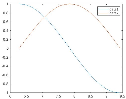
Explanation: As we can see in the above output, we have plotted 2 vectors and our legend function created corresponding labels. Since nothing was passed as an argument to legend function, MATLAB created labels as ‘data1’ and ‘data2’.
Example #2
Now, what if instead of ‘data1’ and ‘data2’, we want to have the name of the function as the label.
Let us learn how to do it.
Our initial code will be the same as in the above example
A = pi : pi/100 : 3*pi
b = cos (A)
c = sin (A)
In addition to the above code, we will add the below-mentioned line:
legend({'sin(A)', 'cos(A)'})
As we can see, we have passed the name of the functions as an argument to our legend function. Here, we can name our functions as per our needs.
This is how our input and output will look like in MATLAB console:
Code:
A = pi : pi/100 : 3*pi

b = cos (A)

c = sin (A)

figure

plot (A, b, A, c)

legend({'sin(A)','cos(A)'})
Output:
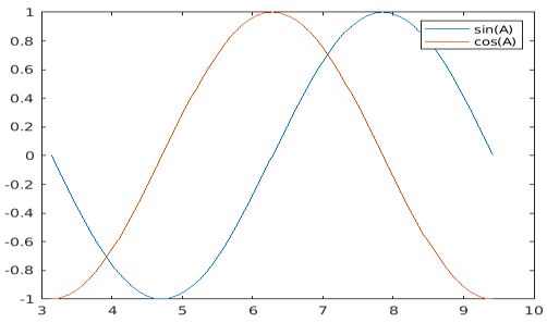
Explanation: Notice on the top right side of the plot, we have got the names of our functions.
Example #3
Next, what if we don’t want our labels to be on the top right but in some other place on the plot.
Let us learn how to achieve that.
Legend function in MATLAB allows us to put our label in place of our choice. All we need to do is pass the pre-defined code for the direction, as an argument.
Our initial code will not change:
A = pi : pi/100 : 3*pi
b = cos (A)
c = sin (A)
In addition to the above code, we will add the below-mentioned line:
legend ({'sin(A)', 'cos(A)'}, 'Location','northwest')
Notice that in addition to the names of the functions, we have added 2 more arguments:
‘Location’ & ‘northwest’. Here ‘Location’ is a keyword for setting the direction of our labels and ‘northwest’ is pre-defined code for direction (Please refer to Table the end of the article to get pre-defined direction codes).
This is how our input and output will look like in MATLAB console:
Code:
A = pi : pi/100 : 3*pi

b = cos (A)

c = sin (A)

figure

plot (A, b, A, c)

legend({'sin(A)','cos(A)'},'Location','northwest')
Output:
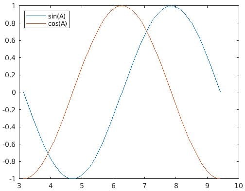
Explanation: As we can clearly see in our output, the label is now on the top left (north west direction).
Example #4
Next, we will learn how to give a name to our label box. i.e we want to convey that sin(A) and cos(A) are our ‘FUNCTIONS’.
Here also our initial code will be the same as above. In addition to that, here we will add the following code:
title(legend,'FUNCTIONS’)
This is how our input and output will look like in MATLAB console:
Code:
A = 2*pi : pi/500 : 3*pi

b = cos (A)

c = sin (A)

figure

plot (A, b, A, c)

legend({'sin(A)','cos(A)'},'Location','northwest')

title(lgd, 'Functions')
Output:
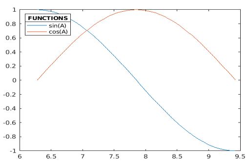
Explanation: As we can notice in the output, our label box is now named.
Conclusion
We learned how to create labels in MATLAB plots and achieve desired styles. We also learned to set the ‘direction’ and ‘Name’ of the label box as per our needs. Labels become very important when we plot multiple functions in the same graph.
Recommended Articles
This is a guide to Matlab Plot Legend. Here we have discussed an introduction to Matlab Plot Legend with appropriate syntax and respective programming examples. You can also go through our other related articles to learn more –
