Updated June 28, 2023

Introduction to Matlab Annotation
Annotating a graph or any document is a very important way to help the readers to understand better context & the argument presented by the graph or document and also to facilitate their understanding of how they should read the graph (or document). Using annotation, we provide any extra information related to the graph that readers might find useful while interpreting the graph. In Matlab, we use ‘annotation’ function for creating various types of annotations.
We have 2 types of annotations in Matlab:
- Line Type
- Shape Type
Syntax:
annotation (lineType, A, B)
annotation (shapeType, dim)
Description:
- annotation (lineType, a, b): It is used to create an arrow or a line annotation. This annotation is extended between the 2 points in the figure.
- annotation (shapeType, dim): It creates a shape annotation of defined size and location.
The ‘lineType’ argument can take the following 4 values:
- Line
- Arrow
- Double Arrow
- Text Arrow
The ‘shapeType’ argument can take the following values:
- Rectangle
- Textbox
Examples of Matlab Annotation
Given below are the examples mentioned:
Example #1
In this example, we will plot a sine wave and then will use line annotation to show the first incident when this sine wave touches the maximum value.
We will follow the following steps:
- Create the sine plot.
- Initialize the points for the annotation line.
- Pass these points as arguments to the annotation function.
Code:
Fs = 0:pi/50:2*pi;
[Defining the frequency for sinewave]y = sin(Fs);
[Initializing the sine wave]plot(Fs,y)
[Creating the plot of sine wave]A = [0.3 0.3];
B = [0.8 0.9];
[Defining the points for the annotation]annotation(‘line,’ A, B)
[Passing the above points to the annotation function]Input:
Fs = 0:pi/50:2*pi;

y = sin(Fs);

plot(Fs,y)

A = [0.3 0.3];

B = [0.8 0.9];

annotation('line', A, B)
Output:
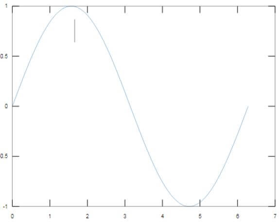
As we can see in the output, the first peak of the sine wave is being pointed out using an annotation line.
Example #2
In this example, we will use the arrow annotation to show the first incident when our sine wave touches the maximum value.
Code:
Fs = 0:pi/50:2*pi;
[Defining the frequency for sinewave]y = sin(Fs);
[Initializing the sine wave]plot(Fs,y)
[Creating the plot of sine wave]A = [0.3 0.3];
B = [0.8 0.9];
[Defining the points for the annotation]annotation(‘arrow,’ A, B)
[Passing the above points to the annotation function. Please note that the first argument in this case is ‘arrow’]Input:
Fs = 0:pi/50:2*pi;

y = sin(Fs);

plot(Fs,y)

A = [0.3 0.3];

B = [0.8 0.9];

annotation('arrow', A, B)
Output:
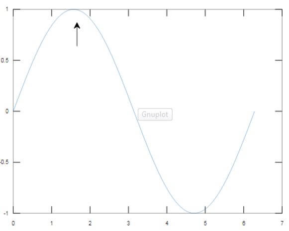
As we can see in the output, the first peak of the sine wave is being pointed out using an annotation arrow.
Example #3
In this example, we will use the double arrow annotation to show the first incident when our sine wave touches the maximum value.
Code:
Fs = 0:pi/50:2*pi;
[Defining the frequency for sinewave]y = sin(Fs);
[Initializing the sine wave]plot(Fs,y)
[Creating the plot of sine wave]A = [0.3 0.3];
B = [0.8 0.9];
[Defining the points for the annotation]annotation(‘doublearrow,’ A, B)
[Passing the above points to the annotation function. Please note that the first argument, in this case, is ‘doublearrow’]Input:
Fs = 0:pi/50:2*pi;

y = sin(Fs);

plot(Fs,y)

A = [0.3 0.3];

B = [0.8 0.9];

annotation('doublearrow', A, B)
Output:
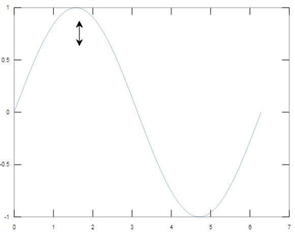
As we can see in the output, the first peak of the sine wave is being pointed out using an annotation double arrow.
All the above annotation types help us to put a line or arrow, but what if we need text also along with the annotation line? For this purpose, we use ‘textarrow’ annotation.
Example #4
In this example, we will use the text arrow annotation to show the first incident when our sine wave touches the maximum value.
Code:
Fs = 0:pi/50:2*pi;
[Defining the frequency for sinewave]y = sin(Fs);
[Initializing the sine wave]plot(Fs,y)
[Creating the plot of sine wave]A = [0.3 0.3];
B = [0.8 0.9];
[Defining the points for the annotation]messageToDisplay = ‘First Maxima’
[Initializing the string with text message]annotation(‘textarrow,’ A, B, ‘String’, str)
[Passing the above points to the annotation function. Please note that the first argument, in this case, is ‘textarrow’.We have also passed the string with a message to be displayed]
Input:
Fs = 0:pi/50:2*pi;

y = sin(Fs);

plot(Fs,y)

A = [0.3 0.3];

B = [0.8 0.9];

messageToDisplay = 'First Maxima'

annotation('textarrow', A, B, 'String', messageToDisplay)
Output:
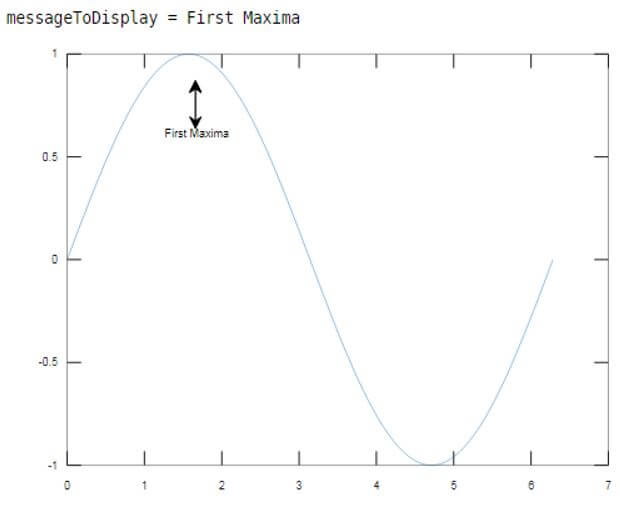
As we can see in the output, the first peak of the sine wave is being pointed, and we also have a text message displayed.
Example #5
In this example, we will use the textbox annotation, which is a shapetype annotation.
Code:
Fs = 0:pi/50:2*pi;
[Defining the frequency for sinewave]y = sin(Fs);
[Initializing the sine wave]plot(Fs,y)
[Creating the plot of sine wave]boxDimension = [0.5 0.5 0.3 0.3];
[Defining the points for the annotation]messageToDisplay = ‘Let us learn annotation’
[Initializing the string with text message]annotation(‘textbox’, boxDimension, ‘String’, messageToDisplay, ‘FitBoxToText,’ ‘on’);
[Passing the above points to the annotation function. Please note that the first argument in this case is ‘textbox’]Input:
Fs = 0:pi/50:2*pi;

y = sin(Fs);

plot(Fs,y)

boxDimension = [0.5 0.5 0.3 0.3];

messageToDisplay = 'Let us learn annotation'

annotation('textbox', boxDimension, 'String', messageToDisplay, 'FitBoxToText', 'on');
Output:
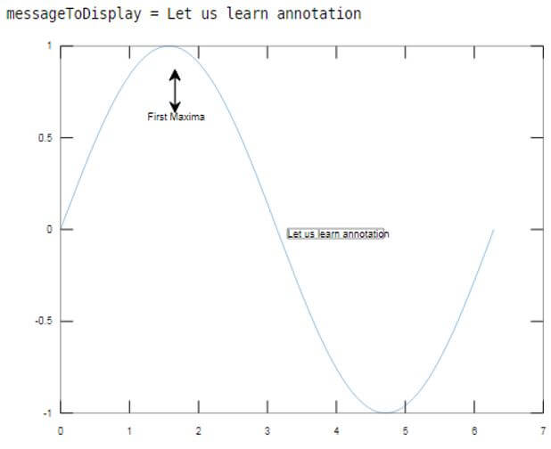
As we can see in the output, our plot has an annotation in the form of a text box with the required message.
To get a simple rectangle as annotation, change the argument from ‘textbox’ to ‘rectangle’ in the above code and remove other arguments.
Conclusion
Annotation is done to make our plot more readable and intuitive. Any additional information that we want the reader to have about our graph can be passed as an annotation. Matlab provides us with various annotation types like line, arrow, textbox, etc.
Recommended Articles
This is a guide to Matlab Annotation. Here we discuss the introduction to Matlab Annotation along with programming examples. You may also have a look at the following articles to learn more –
