Updated June 6, 2023
LOOKUP Formula in Excel
LOOKUP Formula in Excel finds the first column or first row of a table or an array and gives a value from any cell on the same row or column of the table or array, respectively.
Basically, in simple words, this formula helps to search any data from a range of cells or arrays or a table based on its search value. Very quickly and accurately.
Implementation of the LOOKUP Formula
We can implement the LOOKUP Formula in 2 methods.
Method 1
The formula of the LOOKUP function is:
=LOOKUP (lookup_ value, lookup_ vector, [ result_ vector ] )
The arguments for this function are explained in the following table.
| Argument | Explanation |
| Lookup _ Value | The search value is found in the table array’s 1st column or the 1st row. It can either be a text or a Cell Reference. |
| Lookup _ Vector | The search value can be found in the data table’s 1st row or the 1st column. |
| Result _ Vector | The result row, or the result column of the data table, is where the result searched against the Lookup _ Value can be found. |
Method 2
The formula of the LOOKUP function is:
=LOOKUP (lookup_ value, table_ array)
The arguments for this function are explained in the following table.
| Argument | Description |
| lookup_value | It is the search value that is found in the 1st row of the table array. It can either be a text or a Cell Reference. |
| table_array | It refers to the table or array in which you record the result and the search value. Based on the vertical or horizontal table, the 1st column or the 1st row of the selected data range will always be that column or row containing the Lookup _ Value. But in this case, the result will always be from the last column or the last row of the selected data range based on the vertical or horizontal table, respectively. |
How to Use the LOOKUP Formula in Excel?
We will discuss 2 examples of the LOOKUP formula. 1st one is for the data in a Vertical Array, and the later one is for the data in a Horizontal Array.
Example #1
To know about the LOOKUP function, let us take one example.
Tony Stark has a flower shop with a large variety of flowers. Whenever a customer buys a flower, Tony needs to check the price of the flower by looking at every entry in the flower price list.
This wastes a lot of time, as he is required to go through the entire list.
Therefore, he decides to use MS Excel to check the price of the flower.
Tony enters the name of all the flowers in the 1st column. In the 2nd column, he enters the price of each flower.
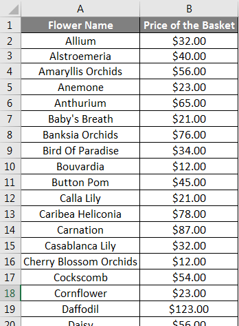
Now he has a list of flowers with their respective prices.
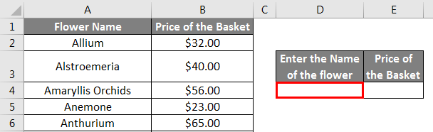
If Tony wants to find the price of any particular flower, he can use the Lookup Function.
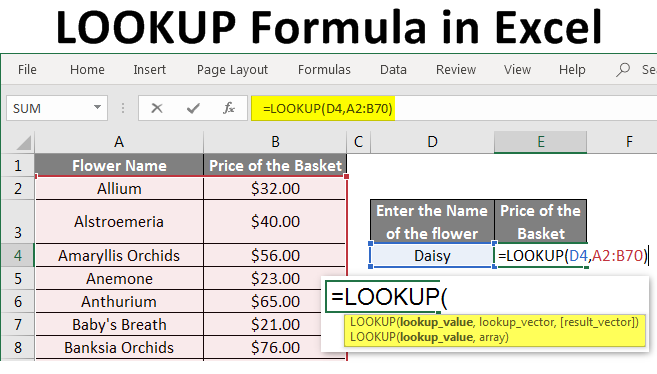
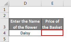
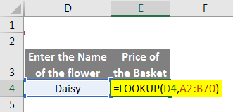
He enters the name of the flower in cell D4. Let us take the name, Daisy.
Then in cell E4, he adds the LOOKUP function, =LOOKUP (D4, A2:B70).
Where,
D4 is the cell that contains the flower name.
A1:B70 is the range, which shall be checked for the flower name and price.
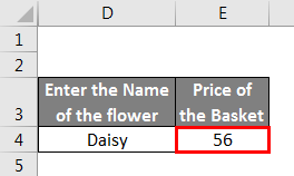
Therefore the price of the entered flower is displayed.
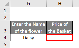
This can also be done in another way, as mentioned earlier.
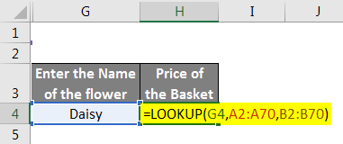
He enters the name of the flower in cell G4. Let us take the name, Daisy.
Then in the H4 cell, he adds the LOOKUP function,
=LOOKUP (G4,A2:A70, B2:B70).
Where,
G4 is the cell that contains the flower name.
A2:A70 is the range, which shall be checked for the flower name.
B2:B70 is the range, which shall be checked for the price of the flower.
Therefore the price of the entered flower is displayed.
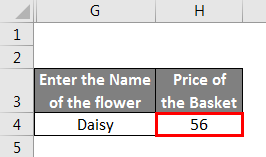
This saves time and effort of Tony.
Example #2
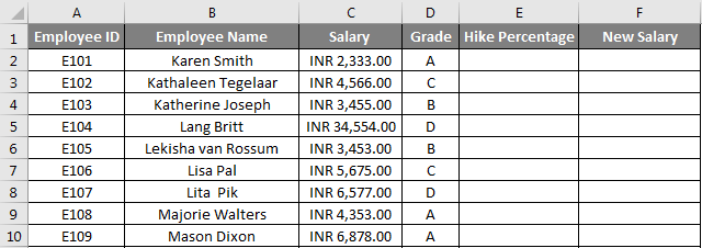
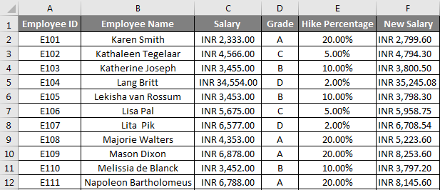
Let us consider the scenario of a GUIDING SOLUTION COMPANY. The Excel worksheet records the employee details, including the Employee’s Name, Salary, and Grade. As per the company’s policy, the annual percentage hike in employees’ salaries will be based on the performance grade.
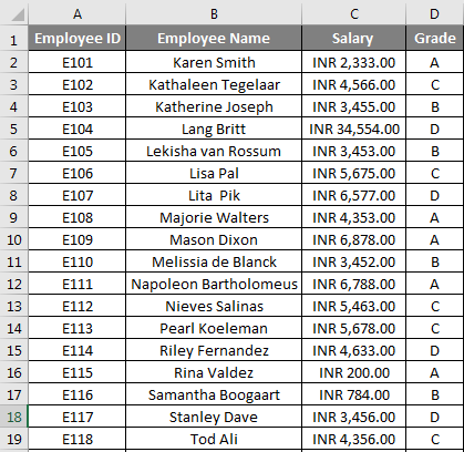
TYouneed to access the incremental details table in the same worksheet. This table contains information about the Grade and its corresponding hike percentage. To fetch the increment applied to the employee.
So now the HR, Steve Rogers, wants to find the Hike Percentage of each employee with the help of the HLOOKUP function. In addition, Steve wants to find out the new salary of each employee.
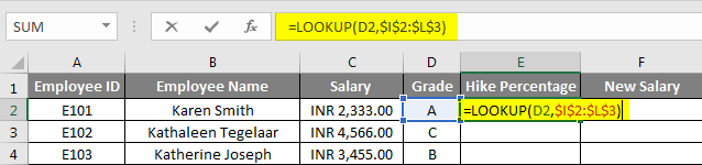
To calculate the hike Percentage, Steve needs to add the LOOKUP function in the E2 cell,
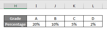
=LOOKUP(D2,$I$2:$L$3)
Where,
D2 is the cell that contains the Grade of each employee
$I$2:$L$3 is the range, which shall be checked for Grade and the Hike Percentage
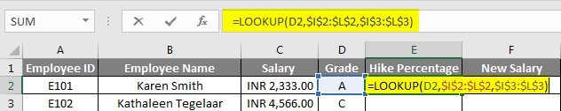
Or Steve can use another way by adding the LOOKUP function in the E2 cell,
=LOOKUP(D2,$I$2:$L$2,$I$3:$L$3)
Where,
D2 is the cell that contains the Grade of each employee.
$I$2:$L$2 is the range, which shall be checked for the Grade
$I$3:$L$3 is the range, which shall be checked for the Hike Percentage.
As a result, the system will display the hike percentage. Then, Steve must drag down the formula to get all the hike percentages of employees according to their grades.
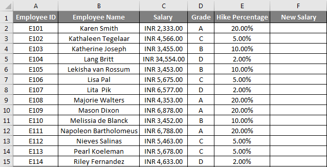
Now Steve needs to find out the new salary after the hike. To accomplish that, he must add the formula =C2+C2*E2.
Where,
C2 is the salary of each employee.
E2 is the Hike percentage based on their Grade.
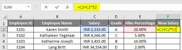
As a result, the new salary will be displayed. Then, Steve must drag down the formula to get the new wages of all the employees after the hike according to their grades.
Things to Remember
- If the selected lookup_value occurs more than once, the LOOKUP function will return the first instance of that lookup_value.
- Lookup_Vector or the table array’s 1st column or 1st row must be in ascending order.
Recommended Articles
This has been a guide to the LOOKUP Formula in Excel. Here, we have discussed How to Use the LOOKUP Formula in Excel, examples, and a downloadable Excel template. You may also look at these helpful Excel articles –
