
Introduction to Linear Regression Analysis
Linear regression analysis is among the most widely used statistical analysis technique as it involves the study of additive and linear relationships between single and multiple variables techniques. The analysis using a single variable is termed the simple linear analysis, while multiple variables are termed multiple linear analysis. Basically, in linear regression analysis, we try to figure out the relationship of the independent and the dependent variables, and that’s why it has multiple advantages such as being simple and powerful in making better business decisions, etc.
3 Types of Regression Analysis
These three Regression analyses have maximum use cases in the real world; otherwise, there are more than 15 types of regression analysis.
Given below are 3 types of regression analysis:
- Linear Regression Analysis
- Multiple Linear Regression Analysis
- Logistic Regression
In this article, we will focus on Simple Linear Regression analysis. This analysis helps us to identify the relationship between the independent factor and the dependent factor. In simpler words, the Regression model helps us find how the independent factor changes affect the dependent factor.
This model helps us in multiple ways like:
- It is a simple and powerful statistical model.
- It will help us in making prediction and forecasts.
- It will help us to make a better business decision.
- It will help us to analyze the results and correcting errors.
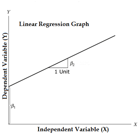
Equation of Linear Regression and Split it into relevant parts:
- Β1 in the mathematical terminology known as intercept and β2 in the mathematical terminology is known as a slope. They are also known as regression coefficients. ϵ is the error term, and it is the part of Y the regression model is unable to explain.
- Y is a dependent variable (other terms which are interchangeably used for dependent variables are response variable, regressand, measured variable, observed variable, responding variable, explained variable, outcome variable, experimental variable, and/or output variable).
- X is an independent variable (regressors, controlled variable, manipulated a variable, explanatory variable, exposure variable, and/or input variable).
Problem: For understanding what is linear regression analysis, we are taking the “Cars” dataset, which comes by default in R directories. In this dataset, there are 50 observations (basically rows) and 2 variables (columns). Columns names are “Dist” and “Speed”. Here we have to see the impact on distance variables due to change speed variables. To see the structure of the data, we can run a code Str(dataset). This code helps us to understand the structure of the dataset. These functionalities help us make better decisions because we have a better picture of the dataset structure. This code helps us to identify the type of datasets.
Code:

Similarly, to check the statistics checkpoints of the dataset, we can use code Summary(cars). This Code provides the mean, median, range of the dataset in a go, which the researcher can use while dealing with the problem.
Output:
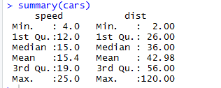
Here we can see the statistical output of every variable we have in our dataset.
Graphical Representation of Datasets
Types of graphical representation which will cover here are and why:
- Scatter Plot: With the help of the graph, we can see in which direction our linear regression model is going, whether there is any strong evidence to prove our model or not.
- Box Plot: Helps us to find outliers.
- Density Plot: Help us understand the independent variable’s distribution; in our case, the independent variable is “Speed”.
Advantages of Graphical Representation
Given below are advantages mentioned:
- Easy to understand.
- It helps us to take quick decision.
- Comparative analysis.
- Less effort and time.
1. Scatter Plot: It will help visualize any relationships between the independent and dependent variables.
Code:
![]()
Output:
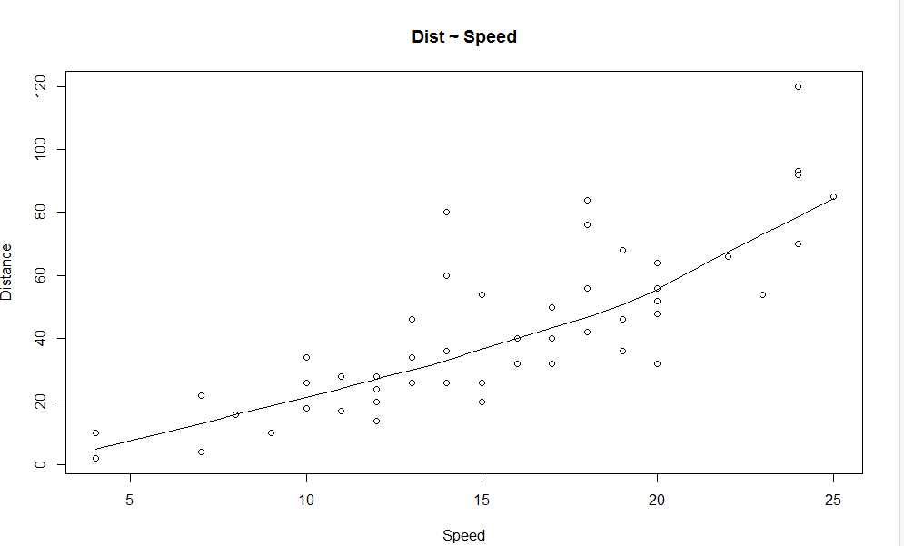
We can see from the graph a linearly increasing relationship between the dependent variable (Distance) and the independent variable (Speed).
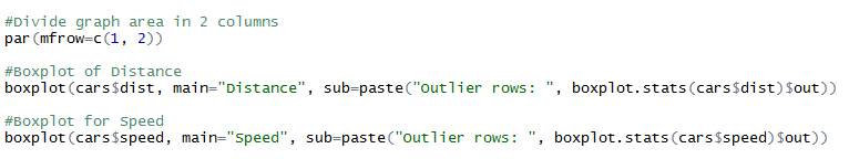
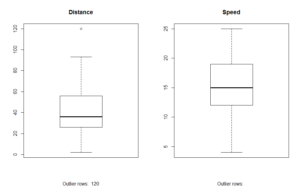
2. Box Plot: Box plot helps us to identify the outliers in the datasets.
Advantages of using a box plot are:
- Graphical display of variables location and spread.
- It helps us to understand the data’s skewness and symmetry.
Code:
Output:
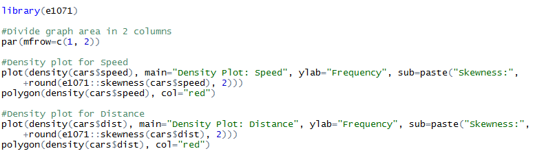
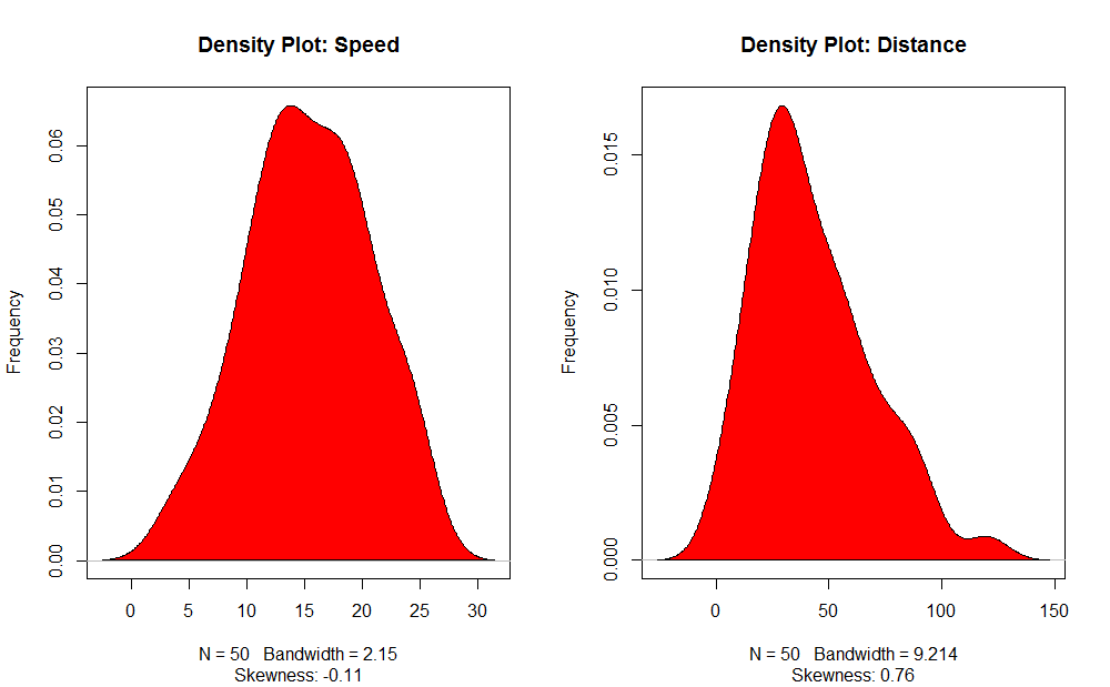
3. Density Plot (to check the normality of the distribution)
Code:
 Output:
Correlation Analysis
This Analysis helps us to find the relationship between the variables.
There are mainly six types of correlation analysis.
- Positive Correlation (0.01 to 0.99)
- Negative Correlation (-0.99 to -0.01)
- No Correlation
- Perfect Correlation
- Strong Correlation (a value closer to ± 0.99)
- Weak Correlation (a value closer to 0)
A Scatter plot helps us to identify which types of correlation datasets have among them, and the code for finding the correlation is
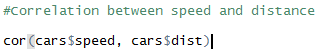
Output:
![]()
Here we have a strong positive correlation between Speed and Distance, which means they directly relate to them.
Linear Regression Model
This is the core component of the analysis; earlier, we were just trying and testing things whether the dataset we have is logical enough to run such analysis or not. The function we are planning to use is lm(). This function contains two elements which are Formula and Data. Before assigning that which variable is dependent or independent, we have to be very sure about that because our whole formula depends on that.
The formula looks like this:
Code:
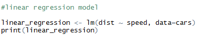
Output:
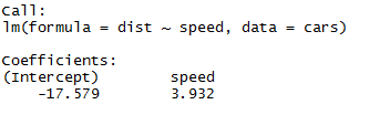
As we can recall from the above segment of the article, the equation of linear regression is:
Now we will fit in the information which we got from the above code in this equation.
Only finding the equation of linear regression is not sufficient; we have to check its statistic significance also. For this, we have to pass a code “Summary” on our linear regression model.
Code:
![]()
Output:
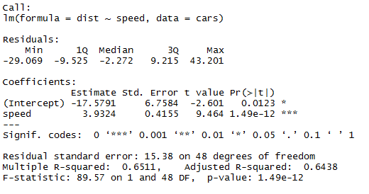
There are multiple ways of checking the statistic significance of a model, and here we are using the P-value method. We can consider a model statistically fit when the P-value is less than the pre-determined statistical significant level, which is ideally 0.05. In our table of summary(linear_regression), we can see that P-value is below the 0.05 level, so we can conclude that our model is statistically significant. Once we are sure about our model, we can use our dataset to predict things.
Recommended Articles
This is a guide to Linear Regression Analysis. Here we discuss the three types of linear regression analysis, the graphical representation of datasets with advantages and linear regression models. You can also go through our other related articles to learn more-