What is the LEFT Formula in Excel?
The LEFT Formula in Excel allows you to extract a substring from a string starting from the leftmost portion of it (that means from the start). It is an inbuilt Excel function specifically defined for string manipulations.
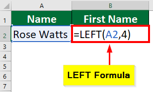
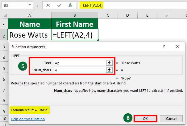
Let’s suppose you have typed the word “Rose Watts” in a cell, and you are interested in extracting just the name “Rose” in another cell. With the LEFT formula, you can achieve this task easily by using the formula “=LEFT(A2, 4)“. In this formula, “A2” signifies the cell containing “Rose Watts” while “4” specifies that you want the first four characters.
Result:
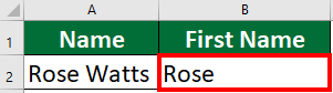
Table of Contents
- What is the LEFT Formula in Excel?
- How to Use LEFT Formula in Excel?
- Can You Use the Left Formula With Dates?
- Left Formula Errors
- Advanced Applications of LEFT Formula in Excel
Now, let’s delve into a more detailed understanding of the LEFT function, starting with its syntax and arguments:
Syntax
=LEFT(text, num_chars)
Arguments
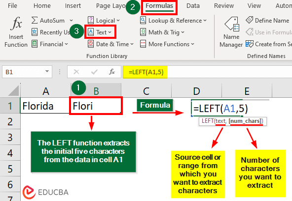
The LEFT formula’s syntax comprises two primary arguments:
- text: This required argument represents the source cell or range from which you want to extract characters.
- num_chars: This argument specifies the number of characters you want to extract from the beginning of the text string. If omitted, the formula extracts only one character.
How to Use LEFT Formula in Excel?
We have two methods to use the LEFT formula in Excel.
A) Direct Cell Formula Approach
- Start typing =LEFT( in the cell where you want to display the result
- Now add the arguments, data and close the bracket like this: =LEFT(A1,2)
- Press Enter, and the result will display in the same cell.
B) Using Excel Ribbon
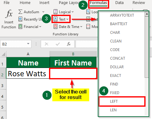
- Select the cell where the result will appear (e.g., B2)
- Go to the Formulas tab
- Find Text in the categories
- Click the LEFT function
- A dialog box will open. Enter the cell (e.g., A2) in Text and the number of characters you want to extract (e.g.,4) in Num_chars
- Click OK to insert the LEFT function
- You can see the result in the bottom left of the dialog box.
Example #1: Extracting a Single Character
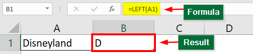
Let’s explore how to utilize the LEFT formula in Excel to extract the initial letter “D” of the word “Disneyland” present in Cell A1.
- Select the cell where you want to display the result (e.g., B2).
- Enter the formula =LEFT(A1) in Cell B2.
- Click Enter.
Result:
We get the result as D.
Example #2: Extracting More than One Character
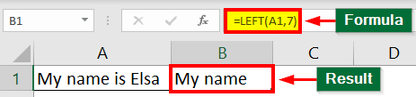
Suppose you have data in cell A1 containing the text “My name is Elsa”, and you need to extract the first 7 characters from this text. Let’s see how to do it using the LEFT formula in Excel:
- Select the destination cell, i.e., B1
- Enter the formula =LEFT(A1,7)
- Press Enter.
Result:
We get the result as “My name.”
Example #3: Extracting Numbers
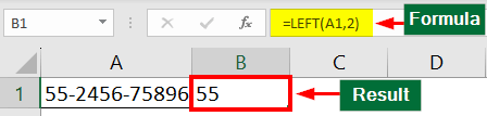
Let us see how we can use the LEFt formula to extract the leftmost numbers from a cell.
- Select Cell B1
- Enter =LEFT(A1,2) as the formula
- Press Enter to display the result.
Result:
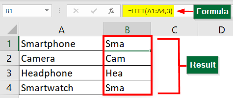
Example #4: Extracting Values for a Range of Cells
Suppose you have a range of cells from A1 to A4, and you want to extract the first 3 characters from each cell. Let’s see how to do that using the LEFT function in Excel.
- Select all the result cells where you want the extracted data, such as B1 to B4
- With these cells selected, enter the formula with a range like this: =LEFT(A1:A4,3)
- Click Ctrl+Shift+Enter for the result.
Result:
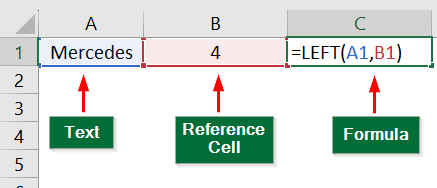
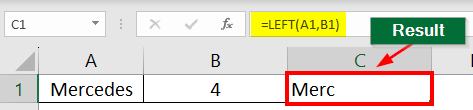
Example #5: Using Cell Reference for Num_chars Argument
Let’s say you have a cell that contains the number of characters you want to extract. Let us see how to use a cell reference in the Num_chars argument.
Given:
Suppose Cell B1 has the value 4. Now, you can use the cell B1 as a cell reference in the LEFT formula to extract the first 4 characters from cell A1. You can use the below formula:
=LEFT(A1,B1)
Result:
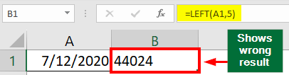
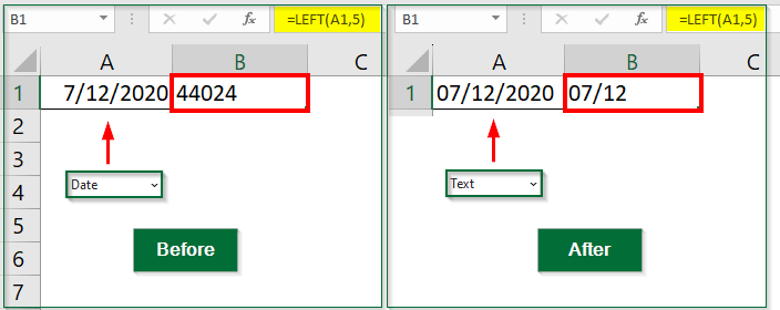
Can You Use the Left Formula With Dates?
It is not possible to use the LEFT formula with dates because dates have a specific format. Excel stores date values as numbers at the backend. Thus, using the LEFT formula on a date in Excel will give you a series of numbers representing the date rather than a part of the date itself.
Therefore, when you use LEFT function on a date:
- You might lose important date details like the day or year.
- Different date formats can give you different results.
- It can lead to errors if dates aren’t in the expected format.
Solution: Change the format of the cell
To work with dates correctly, you can either use functions designed for dates, or you can convert the format of the cell from Date to Text.
As a result, you will be able to extract the date from the cell.
Left Formula Errors
Using the LEFT formula with certain types of characters (non-printable, non-text, etc.) or making any other mistakes can lead to errors. Here are a few errors that can occur while using the LEFT function.
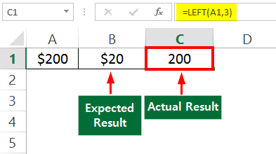
1. LEFT Function does Not Print Non-Text Data
As the LEFT function usually works with text data, it might not work as expected if you use it on dates, or other non-text data (images, audio, binaries, currency, etc). Thus, ensure that the data you are working with is in text or general.
In the image below, when trying to extract the first three characters (“$20”), the function doesn’t account for the dollar symbol. Instead, it shows the following three characters as “200.”
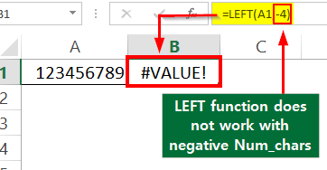
2. #VALUE Error Due to Negative Character Count
If the num_chars argument is not a positive number, i.e., if it’s zero or negative, the LEFT function will return the #VALUE! Error.
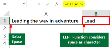
3. Extra Spaces or Non-Printable Characters can affect the result
If there are extra spaces in the text, it can affect the results of the LEFT function.
For instance, in the below image, the text in cell A1 has a single space in the beginning of the sentence. So, when we try to extract 5 characters, we get the result as “ Lead” rather than “Leadi”.
Advanced Applications of LEFT Formula in Excel
Apart from using the LEFT function on its own, we can combine the LEFT function with other functions for more advanced applications.
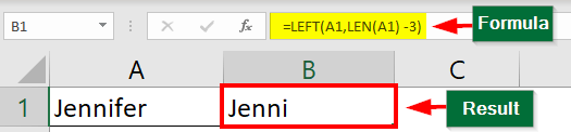
1. LEFT with LEN Function
Let’s say you have the text string in cell A1 and you want to remove the last 3 characters, we can use the combination of LEFT and LEN functions:
=LEFT(A1, LEN(A1) – 3)
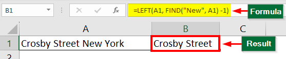
2. LEFT with FIND Function
Let’s say, you want to extract text from cell A1 up to “New”. You can use the below formula:
=LEFT(A1, FIND(“New”, A1) – 1)
Result:
This formula finds the position of the “New” using FIND, then extracts the desired text using LEFT.
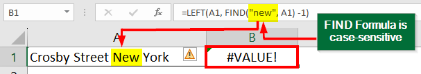
💡Note: The FIND function is case-sensitive when searching for text within a cell. Thus, make sure to write the word in the proper case.
For example, if you put “New” in lowercase, then it will show a #VALUE! Error.
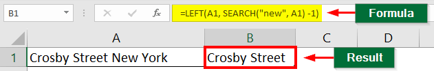
3. LEFT with SEARCH Function
The LEFT with SEARCH formula works the same way as LEFT with FIND. The only difference is SEARCH is not case-sensitive.
For instance, when you use SEARCH, it will find the desired text regardless of whether it’s written as “new,” “NEW,” or “New,” focusing only on the term “New.”
4. LEFT with VALUE Function
Let us take an example of a cell that has alphanumeric values. Suppose we want to display the first three characters in a number format. If we simply use the LEFT formula, we will get the result in text format not number format.
Thus, we can use the LEFT function with the VALUE function and convert the characters into numerical format.
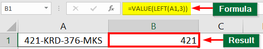
💡Note: In the above image, the content in cell A1 is in text format while the numbers in cell B1 are in number format.
Frequently Asked Questions (FAQs)
Q1. What are the other softwares in which we can use the LEFT function?
Answer: Apart from Excel, you can use the LEFT function in various software and programming languages, including:
- Tableau
- Power BI
- DAX (Data Analysis Expressions)
- SQL (Structured Query Language)
- JavaScript
These tools and languages provide the LEFT function to manipulate and extract characters from text strings similarly across different platforms.
Q2. Does the LEFT function work similarly to Excel in Google Sheets?
Answer: Yes, the LEFT function works similarly in Google Sheets as it does in Excel. It extracts characters from the start of a text string, and its usage is consistent between the two programs.
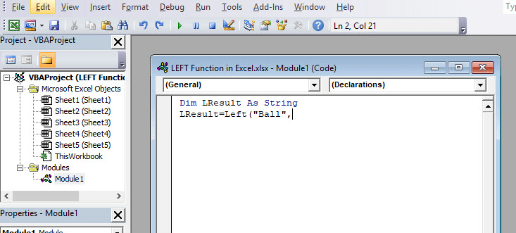
Q3. Can you use the LEFT function with Excel VBA?
Yes, we can use the LEFT formula with VBA, for which you can use the Microsoft Visual Basic Editor.
You can either give sheet reference for the source cell or enter the word directly, as shown below,
=LEFT(“Ball”,1)
Recommended Articles
This article is a guide to the LEFT formula in Excel. Here we discuss how to use the LEFT function in Excel using several examples. We have also provided a downloadable Excel template. You can also go through our other suggested articles,
