


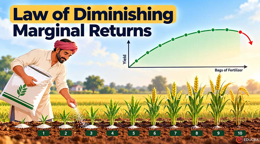
Imagine a wheat farmer near Ludhiana preparing his one-hectare field for the winter crop. After sowing in November, he applies urea fertilizer to help the young wheat plants grow. The first few bags make a noticeable difference, helping the crop grow greener and produce more grain.
But adding more fertilizer does not guarantee a bigger harvest. By the time he applies the tenth bag, the extra nitrogen may do more harm than good, reducing his yield even though it costs the same ₹266.50 as the first bag.
This illustrates the law of diminishing marginal returns, an economic principle that explains why adding more of one input eventually produces smaller gains when other factors remain unchanged. The same idea applies beyond farming, from hiring extra workers at a busy dosa stall to spending additional hours studying for an exam.
How the Law of Diminishing Marginal Returns Works?
The law of diminishing marginal returns requires changing one input while everything else stays constant. The farmer’s hectare and winter weather remain the same, and only the number of urea bags changes. Going from three bags to four lifts his yield from 4,520 kg to 4,860 kg. The marginal product formula measures the change in output divided by the change in input; the fourth bag adds 340 kg of wheat. Bag by bag, that figure falls from the second bag onward, while the total harvest keeps climbing until bag nine.
Students often misunderstand the law of diminishing marginal returns because they hear “diminishing” and picture a falling harvest. The farmer’s sixth bag still adds 190 kg of wheat, though that is less than the 260 kg the fifth bag contributed. The total harvest only starts shrinking at the far end, when the extra input begins to cause harm. Textbooks divide the production curve into stages of increasing, diminishing, and negative returns. Almost every bag on the farmer’s hectare falls in the middle stage.
Agronomists measure the plant’s response using a ratio called nutrient use efficiency, which represents the kilograms of grain produced per kilogram of nitrogen applied. The farmer’s first bag achieves about 29 kg of grain per kilogram of nitrogen. Later bags deliver far lower returns, mainly because the wheat may run short of root space or water before it runs short of nitrogen. The extra nitrogen then remains in the soil or becomes vulnerable to losses. Much fertilizer research focuses on improving nutrient uptake through better timing and slow-release products, helping more nutrients reach the crop before returns decline. Split applications are practical: apply some urea at sowing and reserve the rest for when the crop is growing fastest.
Ten Bags on One Hectare
These yields are invented and rounded, so read them as a teaching curve, not a Ludhiana forecast. Real trials bounce around far more, and a hot March can drag the whole curve down, as Punjab’s growers found in 2022. Harjeet starts from 3,000 kg with no urea, and since urea is 46% nitrogen, each 45 kg bag carries about 20.7 kg of N.
| Bags Applied | Total Yield (kg) | Extra Grain From That Bag (kg) |
| 0 | 3,000 | baseline |
| 1 | 3,600 | 600 |
| 2 | 4,100 | 500 |
| 3 | 4,520 | 420 |
| 4 | 4,860 | 340 |
| 5 | 5,120 | 260 |
| 6 | 5,310 | 190 |
| 7 | 5,430 | 120 |
| 8 | 5,490 | 60 |
| 9 | 5,500 | 10 |
| 10 | 5,460 | -40 |
Farmers comparing notes tend to quote the middle column. However, the right-hand column better illustrates the law of diminishing marginal returns. It begins with 600 kg of additional wheat from the first bag alone. By the ninth bag, the gain has fallen to just 10 kg, or less than half a kilogram of wheat per kilogram of nitrogen. Such a small increase may be difficult to distinguish from normal field variation once the grain is harvested.
The tenth bag reduces the total yield by 40 kg. Applying excessive nitrogen can encourage tall growth and weaken the crop’s ability to remain upright, increasing the risk of lodging. A March hailstorm or strong wind can flatten the crop across a field, making lodged wheat harder to harvest and potentially reducing grain quality.
The tenth bag is an easy decision to reject in this example. The harder decisions involve bags five through nine, because each still increases total output and may appear worthwhile. Whether the additional fertilizer actually makes financial sense depends on grain prices and fertilizer costs. The marginal benefit formula helps compare the value of one additional unit with its associated cost. Total output alone cannot determine the most profitable input level.
Applying the Law of Diminishing Marginal Returns to Profit
The farmer’s fertilizer and wheat prices illustrate how the law of diminishing marginal returns affects production decisions. Urea’s official price has been ₹242 for a 45 kg bag since the government reduced the bag size from 50 kg in 2018, while farmers may pay around ₹266.50 after applicable charges. A minister told the Lok Sabha in March 2026 that the government had no plan to raise the price. The Union Cabinet set wheat’s minimum support price for the 2027–28 marketing season, when a crop sown in November 2026 would be sold, at ₹2,610 per quintal on September 30, 2026, just ₹25 above the previous year’s rate. That equals approximately ₹26.10 per kilogram.
At those prices, his first bag brings back ₹15,660 worth of wheat. Bag eight still returns about ₹1,570. Bag nine, at roughly ₹260, falls just short of its ₹266.50 cost, so on these numbers the profit peak lands on bag eight, one bag and 10 kg short of the yield peak. When a bag of fertilizer is this cheap next to the grain it grows, price does very little to hold the rate down, and only bag ten loses money by any real margin. Nitrogen the crop never takes up does not disappear, either; some of it leaches toward groundwater as nitrate, a cost that never shows up on Harjeet’s bill.
Change one number and the answer moves. Suppose, as a thought experiment, the same bag cost ₹2,000. Bag seven, worth ₹3,132 of wheat, still pays, but bag eight’s ₹1,566 does not, so Harjeet would stop at seven bags and leave 70 kg of possible grain in the field on purpose.
In the US Corn Belt, extension advice already works this way. Agronomists in seven states set corn nitrogen recommendations using a method called maximum return to nitrogen, which lands below the yield-maximizing rate by design. In a 2022 Crops & Soils explainer, Emerson Nafziger and three co-authors show the recommended rate for central Illinois corn dropping from 181 to 141 pounds of nitrogen an acre as nitrogen rose from $0.50 to $1.25 a pound, with corn held at $5 a bushel. Their write-up states the result plainly: “The MRTN N rate decreased as N cost rose,” then gives the two rates.
Real-World Examples of the Law of Diminishing Marginal Returns
The principle applies far beyond agriculture. When returns begin to flatten, people and businesses often respond by adding more of the same input. However, the real constraint may be another resource that does not change.
Consider a hypothetical dosa stall in Bengaluru with one large tawa on a busy Sunday morning. Hiring a third cook may barely shorten the queue when the tawa already holds as many dosas as two people can turn efficiently. A fourth cook adds labor without increasing the cooking surface’s capacity. The stall experiences diminishing marginal returns because equipment, not the number of workers, limits production.
Exam preparation follows a similar pattern. For a Class 12 student, the third hour of revision after midnight may cover far less material than the first hour after dinner. A fourth hour may contribute little if fatigue reduces concentration and recall. Alertness is the limiting factor. Moving the study session to the next morning may improve productivity because it addresses the constraint rather than adding more hours.
The law of diminishing marginal returns also influenced early economic thinking. Economists once feared that population growth would permanently reduce output per person because farmland had limited productive capacity. Britannica’s explanation of diminishing returns notes that the principle is particularly relevant to economies where technology changes slowly, while technological improvements can alter the outcome.
Punjab offers a useful illustration. Semi-dwarf wheat, developed from Norman Borlaug’s Mexican breeding lines, arrived in the mid-1960s, and expanding irrigation helped farmers get much higher yields from existing farmland. These developments show why diminishing returns do not mean productivity can never improve. New technology, better inputs, improved farming methods, or more efficient resource use can shift the production curve upward. When an additional input stops delivering worthwhile gains, it is worth examining which other factors have been treated as fixed.
Final Thoughts
The farmer’s tenth bag of urea costs the same as his first, yet it reduces his harvest in the illustrative example. The key measure is not total output but the additional output from the last unit of input, relative to its cost.
At ₹266.50 per bag and ₹26.10 per kilogram of wheat, the example suggests the farmer should stop at eight bags to maximize profit, even though nine yield the largest harvest. If fertilizer prices rise, the profitable application rate can fall further.
The law of diminishing marginal returns helps a business, farmer, or student decide whether to add more of a resource. The next unit is worthwhile only when its expected benefit exceeds its cost, while environmental effects and other constraints may also influence the decision. Before adding more fertilizer, labor, or study time, compare the return from the last unit with what it costs. That calculation can reveal when more is no longer better.
Recommended Articles
Explore related economics concepts to understand marginal product, marginal benefit, and how businesses make efficient production decisions. Learn how the law of diminishing marginal returns influences costs, productivity, and profit maximization.