Introduction to Kruskal’s Algorithm in C
Kruskal’s Algorithm, conceived by Joseph Kruskal in 1956, stands as a cornerstone in graph theory, particularly for determining the minimum spanning tree (MST) of a connected, undirected graph. The MST, vital for establishing an optimal network of connections while minimizing the overall weight of edges and ensuring the absence of cycles, is systematically constructed through the algorithm’s iterative process. By sorting edges based on their weights and progressively incorporating them into the tree if they do not create cycles, Kruskal’s Algorithm efficiently navigates through the graph to produce an optimal solution.
In implementing this algorithm in the C programming language, direct attention towards effectively managing the graph’s representation, sorting edges, and detecting cycles using suitable data structures and algorithms. The algorithm’s modular design facilitates independent development and integration of various components, such as sorting mechanisms, data structures, and traversal methods, as well as customization of the solution to diverse applications and scenarios, resulting in a robust and versatile solution.
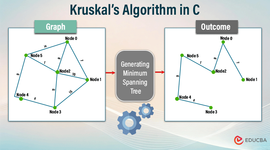
Table of Contents
Understanding Kruskal’s Algorithm
Understanding Kruskal’s algorithm entails grasping its greedy nature, understanding the importance of sorting edges, the cycle detection mechanism, and the role of the disjoint-set data structure in ensuring efficiency and correctness.
Minimum Spanning Tree (MST):
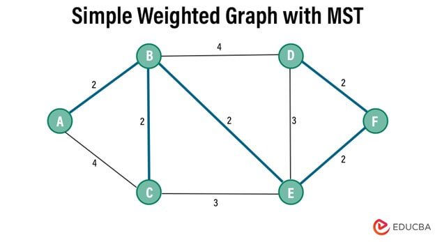
An essential concept in graph theory, especially for connected, undirected graphs, is the minimum spanning tree (MST). In a graph with weighted edges, the MST is a subset of edges that accomplishes the following:
- It connects all vertices within the original graph.
- It forms a tree structure, meaning it’s devoid of cycles.
- It minimizes the total weight of edges compared to all other possible spanning trees. In essence, the MST represents the most efficient means of connecting all vertices while reducing the overall edge weight.
Example:
Output: 10
Step-by-Step Explanation
Kruskal’s Algorithm, a popular approach for determining the MST of a graph, follows these steps:
- Initially, arrange all edges in the graph in ascending order of weight.
- We establish an empty set to collect the Minimum Spanning Tree (MST) edges.
- The algorithm proceeds through the sorted edges, starting with the lightest.
- For each edge, it verifies if adding it to the MST set would form a cycle, employing a disjoint-set data structure (often known as Union-Find).
- If the addition of the edge does not result in the formation of a cycle, it becomes part of the MST set.
- This process repeats until all vertices are interconnected, culminating in the construction of the MST.
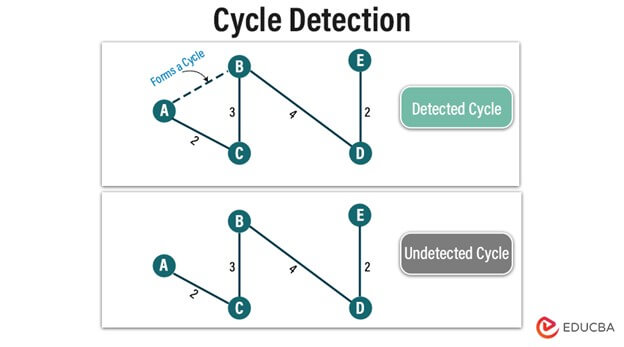
Key Concept: Cycle Detection
In Kruskal’s Algorithm, detecting cycles is vital to ensure the resulting tree is free of cycles. Achieve this using the disjoint-set data structure (Union-Find), which manages disjoint sets of vertices and facilitates efficient union and find operations. When assessing whether to add an edge to the MST, Kruskal’s Algorithm employs Union-Find to check for cycles. Through union operations and tracking connected components, it swiftly identifies cycles incorporating only acyclic edges into the MST. This robust mechanism guarantees the algorithm’s correctness and ensures the creation of a valid minimum spanning tree.
Pseudocode of Kruskal’s Algorithm
function Kruskal(graph):
  // Create a forest (collection of disjoint sets)
  forest = []
  for vertex in graph.vertices:
    forest.append({vertex})

  // Sort edges by weight in ascending order
  edges = graph.edges.sort(key=lambda edge: edge.weight)

  // Loop through edges
  for edge in edges:
    u, v = edge.source, edge.target  // Get source and target vertices

    // Check if adding edge creates a cycle
    if find(forest, u) != find(forest, v):
      // No cycle, merge sets and add edge to forest
      union(forest, u, v)
      forest.append(edge)

  return forest

function find(forest, vertex):
  // Find the root of the set containing the vertex
  while vertex != forest[vertex].parent:
    vertex = forest[vertex].parent
  return vertex

function union(forest, u, v):
  // Find roots of sets containing u and v
  root_u = find(forest, u)
  root_v = find(forest, v)

  // Attach smaller tree under root of larger tree
  if forest[root_u].rank < forest[root_v].rank:
    forest[root_u].parent = root_v
  else:
    forest[root_v].parent = root_u
    if forest[root_u].rank == forest[root_v].rank:
      forest[root_u].rank += 1
This pseudocode uses two helper functions:
- find(forest, vertex): Finds the root of the set containing the vertex in the forest.
- union(forest, u, v): Merges the sets containing vertices u and v by attaching the smaller tree under the root of the larger tree. It also uses the concept of rank to optimize union operations.
Implementation in C
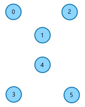
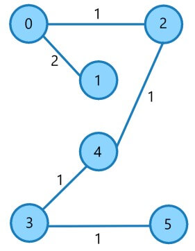
Input Graph:
Code Implementation:
#include
#include
// Structure to represent an edge in the graph
struct Edge {
int source;
int target;
int weight;
};
// Structure to represent a subset for union-find
struct subset {
int parent;
int rank;
};
// Function to compare two edges by weight
int compare(const void* a, const void* b) {
struct Edge* e1 = (struct Edge*)a;
struct Edge* e2 = (struct Edge*)b;
return e1->weight > e2->weight;
}
// Function to create a new subset with a single element
struct subset* createSubset(int vertex) {
struct subset* subset = (struct subset*)malloc(sizeof(struct subset));
subset->parent = vertex;
subset->rank = 0;
return subset;
}
// Function to find the root of the set the vertex belongs to
int find(struct subset subsets[], int vertex) {
if (subsets[vertex].parent != vertex)
subsets[vertex].parent = find(subsets, subsets[vertex].parent);
return subsets[vertex].parent;
}
// Function to perform union of two sets
void Union(struct subset subsets[], int x, int y) {
int xroot = find(subsets, x);
int yroot = find(subsets, y);
// Attach smaller rank tree under root of larger rank tree
if (subsets[xroot].rank < subsets[yroot].rank) subsets[xroot].parent = yroot; else if (subsets[xroot].rank > subsets[yroot].rank)
subsets[yroot].parent = xroot;
else {
subsets[yroot].parent = xroot;
subsets[xroot].rank++;
}
}
// Function to construct MST using Kruskal's algorithm
void KruskalMST(struct Edge edges[], int V, int E) {
// Sort edges by weight
qsort(edges, E, sizeof(edges[0]), compare);
// Allocate memory for subsets
struct subset* subsets = (struct subset*)malloc(V * sizeof(struct subset));
// Create V subsets with single elements
for (int i = 0; i < V; ++i)
subsets[i] = *createSubset(i);
// Include edges in MST
int edge_included = 0;
int i = 0;
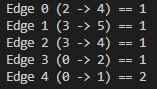
while (edge_included < V - 1) { struct Edge currentEdge = edges[i++]; int x = find(subsets, currentEdge.source); int y = find(subsets, currentEdge.target); // Check if adding edge creates a cycle if (x != y) { printf("Edge %d (%d -> %d) == %d\n", edge_included, currentEdge.source, currentEdge.target, currentEdge.weight);
Union(subsets, x, y);
edge_included++;
}
}
// Free memory allocated for subsets
free(subsets);
}
int main() {
int V = 6; // number of vertices
int E = 9; // number of edges
struct Edge edges[] = {
{0, 1, 2}, {0, 3, 4}, {1, 2, 3}, {1, 4, 4}, {2, 4, 1}, {3, 4, 1}, {3, 5, 1}, {4, 5, 2}, {0, 2, 1}
};
KruskalMST(edges, V, E);
return 0;
}Output
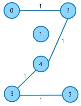
Output Graph:

Data Structures:
A disjoint-set data structure, also known as Union-Find, is a fundamental data structure used in Kruskal’s Algorithm to detect cycles efficiently and maintain the connected components of a graph.
Disjoint-set Data Structure (Union-Find)
The Disjoint-set data structure manages separate sets without overlapping elements and supports two primary operations: Union and Find.
- Union: This merges two sets, combining their elements into a single set. Typically, Union includes optimizations, such as union by rank or size, to improve efficiency.
- Find: This locates the set to which an element belongs, identifying the set’s representative element (or root) that contains the given element.
Application in Kruskal’s Algorithm
In Kruskal’s Algorithm, the disjoint-set data structure efficiently identifies cycles when adding edges to the minimum spanning tree (MST). Before incorporating an edge into the MST, the algorithm employs the Find operation to ascertain whether the edge’s endpoints belong to the same set. If they are part of different sets, signifying that adding the edge won’t create a cycle, the Union operation combines the sets. Conversely, if adding the edge would result in a cycle, it is omitted from consideration.
Testing and Debugging
1. Tabular Representation
| Edge No. | Vertex Pair | Edge Weight |
| E1 | (0,2) | 1 |
| E2 | (2,4) | 1 |
| E3 | (3,4) | 1 |
| E4 | (3,5) | 1 |
| E5 | (0,1) | 2 |
| E6 | (4,5) | 2 |
| E7 | (1,2) | 3 |
| E8 | (0,3) | 4 |
| E9 | (1,4) | 4 |
2. Step by Step Walkthrough
Graph
Edge 0
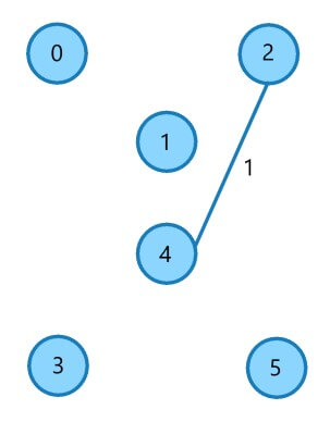
Edge 1

Edge 2
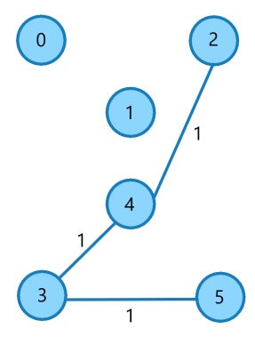
Edge 3
Edge 4
Complexity Analysis
Kruskal’s Algorithm primarily involves sorting edges and performing union-find operations. Therefore, its time complexity depends on the following factors:
- Sorting:
Sorting the edges based on weight usually demands O(E log E) time complexity, utilizing efficient sorting algorithms such as Quick Sort or Merge Sort. In this context, ‘E’ represents the number of edges present in the graph.
- Union-Find Operations:
The time complexity of union-find operations relies on the specific implementation and optimizations applied. In the worst-case scenario, these operations may have an O(log V) time complexity, where V signifies the number of vertices in the graph. Considering Kruskal’s Algorithm executes union-find operations for every edge, the overall time complexity for these operations amounts to O(E log V).
- Overall Time Complexity:
The sorting step is the main factor determining the overall time complexity of Kruskal’s Algorithm, which dominates the algorithm’s performance. Typically, we express the algorithm’s time complexity as O(E log E) or O(E log V), depending on which value, E or V, is larger.
Optimization Consideration
- Path Compression in Union-Find:
Integrating path compression into the union-find data structure. This technique involves adjusting the parent pointers of all elements traversed during a Find operation to point directly to the root. Consequently, it diminishes the tree’s height, enhancing the efficiency of union-find operations overall.
- Union by Rank or Size:
Incorporating the union by rank or size heuristic into union-find operations provides additional efficiency. These strategies prioritize merging smaller sets into larger ones during union operations, effectively preventing significant increases in tree height and ensuring a balanced structure.
- Efficient Sorting Algorithms:
Employing efficient sorting algorithms like Merge Sort or Quick Sort to organize edges by weight mitigates the algorithm’s overall time complexity. Selecting a suitable sorting algorithm based on the graph’s characteristics can substantially boost performance.
- Early Termination:
Implementing early termination strategies can enhance runtime performance. For instance, terminating the algorithm once the MST contains V-1 edges (where V represents the number of vertices) helps avoid unnecessary edge comparisons, particularly in graphs with numerous edges.
- Sparse Graph Optimization:
In scenarios with sparse graphs, where the number of edges is notably smaller than the maximum possible (V^2 for a graph with V vertices), leveraging data structures optimized for sparse graphs, such as adjacency lists, reduces memory consumption and enhances overall efficiency. Additionally, employing algorithms tailored for sparse graphs, like Borůvka’s algorithm, may offer improved efficiency in such contexts.
Real World Applications
- Network Design:
Engineers extensively use Kruskal’s algorithm to devise streamlined network architectures, such as telecommunications. It aids in strategically deploying communication infrastructure and optimizing the placement of cables or transmission lines across diverse locations to minimize costs or distances.
- Circuit Design:
Within electronic circuitry, Kruskal’s Algorithm proves invaluable for optimizing component interconnections. Determining the most efficient layout for wiring between elements reduces overall wire length in circuit boards, thus reducing manufacturing expenses and enhancing operational efficiency.
- Transportation Planning:
Transportation networks encompassing roads, railways, and air routes leverage Kruskal’s Algorithm to chart the most economical links between destinations. This approach streamlines transportation infrastructure, enhancing efficiency and decreasing travel durations.
- Spanning Tree Protocols in Computer Networks:
Kruskal’s Algorithm forms the backbone of Spanning Tree Protocols (STP) in computer networks like Ethernet. These protocols, akin to Kruskal’s Algorithm, craft loop-free network topologies, ensuring seamless data transmission without the risk of network loops.
- Power Distribution Networks:
Kruskal’s Algorithm finds application in optimizing power distribution grids, such as electrical networks. Determining the most efficient pathways to connect power generation stations with end-users minimizes these networks’ energy losses and operational costs.
- Water Distribution Systems:
Municipal authorities rely on Kruskal’s Algorithm to design water distribution networks efficiently. It aids in strategically routing water from treatment facilities to residential and commercial areas, thereby reducing energy consumption and upkeep expenses.
- Optical Fiber Networks:
Kruskal’s Algorithm plays a vital role in shaping the layout of optical fiber networks in telecommunications infrastructure. Identifying the optimal routes for laying fiber optic cables facilitates the connectivity of data centers, service providers, and end-users, ensuring robust communication pathways.
Conclusion
Kruskal’s Algorithm is a pivotal tool within graph theory and optimization, renowned for its efficiency in constructing minimum-spanning trees. The algorithm holds relevance across various domains, including network design, transportation planning, and power distribution, by systematically selecting edges based on their ascending weights. Its straightforward approach and proficiency in resolving intricate connectivity challenges accentuate its practical utility in real-world applications. As technological advancements persist, Kruskal’s Algorithm stands as a linchpin, facilitating the development of resilient and streamlined infrastructures that foster advancement and ingenuity.
Frequently Asked Questions (FAQs)
Q1. When should I use Kruskal’s Algorithm?
Answer: Kruskal’s Algorithm is well-suited for discovering the minimum spanning tree of an undirected graph featuring weighted edges. Its efficacy shines in scenarios where the graph exhibits density or when edge weights are modest compared to the vertex count.
Q2. Can Kruskal’s Algorithm handle graphs with negative edge weights?
Answer: No, Kruskal’s Algorithm cannot handle graphs with negative edge weights. The algorithm relies on sorting edges in the non-decreasing order of their weights, and negative edge weights may result in inaccurate outcomes or infinite loops.
Q3. What happens if the input graph is not connected?
Answer: When the input graph lacks connectivity, Kruskal’s Algorithm generates a minimum-spanning forest rather than a singular minimum-spanning tree. This forest comprises multiple minimum-spanning trees, each representing a connected component within the graph.
Recommended Articles
We hope that this EDUCBA information on “Kruskal’s Algorithm in C” was beneficial to you. You can view EDUCBA’s recommended articles for more information,