Updated June 9, 2023
Excel NORMSINV (Table of Contents)
Introduction to Excel NORMSINV
The NORMSINV function in Excel calculates the probability of inverse normal cumulative distribution, which has a mean and standard deviation. Normsinv function can be seen as Norm.S.Inv. To find NORMSINV, first, we need to calculate the Normal Distribution; we must have X, Mean, and Standard Deviation. Once we get the value of Normal Distribution, we can easily calculate NORMSINV using the probability we got as per syntax.
Syntax of Excel NORMSINV
Argument:
Probability – Which is nothing but probability corresponds to the normal distribution.
How to Use NORMSINV Formula in Excel?
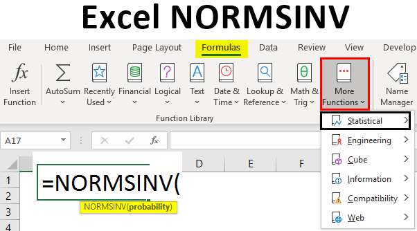
Microsoft Excel categorizes the NORMSINV built-in function under the statistical function. This is illustrated in the screenshot below, which calculates the inverse of the normal cumulative distribution for a given probability.
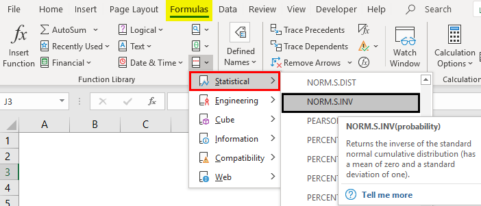
- Go to Formulas Menu.
- Click More Function as shown in the below screenshot.
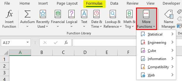
- Choose a Statistical category under that we will find the NORM. The DIST function is shown below.
Example #1 – Using NORM.DIST and NORMSINV
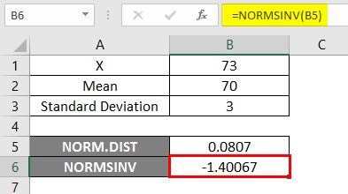
To use NORM.DIST function, let’s start with an easy example where we need to find out the Student’s Grades; suppose we have the class exam with an average grade of 70, i.e., mu=70 and class standard deviation is 3 Points, i.e., sigma=3 here we need to find out what is the probability that students got the marks 73 or below, i.e., P(X<=73). So let’s see how to find out the probability using the NORM.DIST function.
- X=3
- Mean=70
- Standard Deviation=3
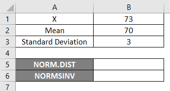
- Apply the NORM.DIST function as below.
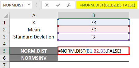
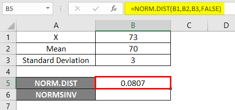
- Suppose we apply the above NORM.DIST function, we will get the probability of 0.0807.
- Now apply the NORMSINV function to find the inverse of the normal cumulative distribution, as shown below.
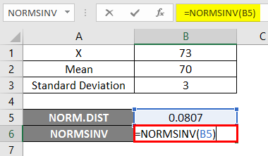
Result –
In the below result, we can see that we got negative values -1.40067 for the given probability, i.e., the inverse of normal cumulative distribution.
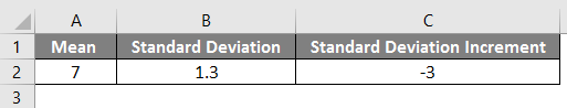
Example #2 – Mean and Exact Standard Deviation
Let’s see another example with curve-based data to get to know the mean and exact standard deviation.
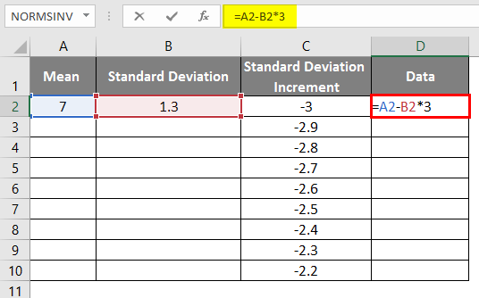
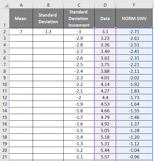
- Mean =7
- Standard Deviation=1.3
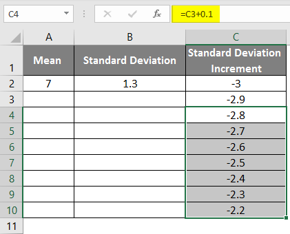
- Standard Deviation Increment as -3
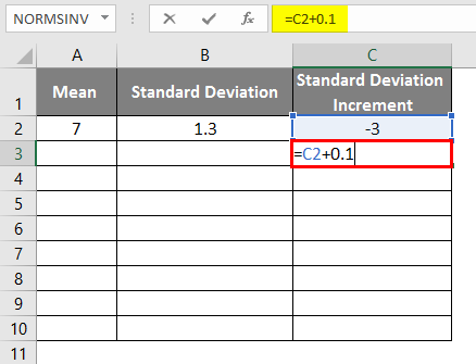
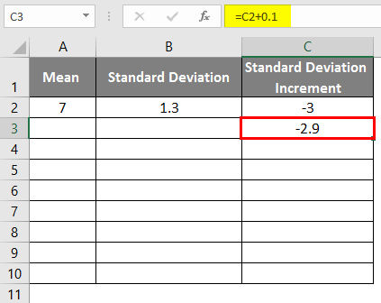
- To get the bell curve, we have to add a 0.1 to standard deviation increment where the data is shown below.
- After applying the formula, the result is shown below.
- Drag the values to get more ones until we get the positive ones to get a left curve.
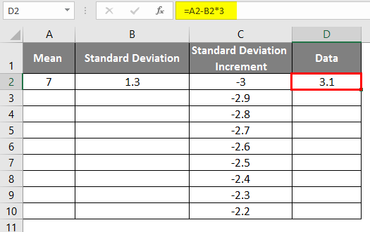
- We must apply the formula as =mean-standard deviation * 3 to get the exact curves to get the right curve.
- After using the formula, the result is shown below.
- As in the above data for standard deviation increment to get the left curve, we have incremented the values by 0.1
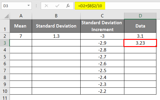
- The same scenario is used by applying the formula as =3.1+STANDARD DEVIATION/10 to get the curve increment of 0.1
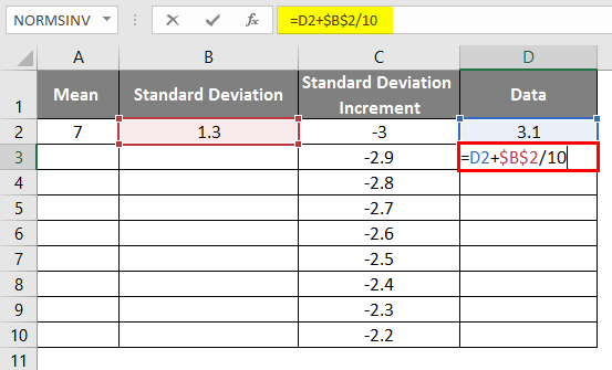
- After using the formula, the result is shown below.
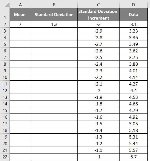
- Drag the values to get the exact result shown in the screenshot below.
- Now apply the normal distribution function with the formula = NORM.DIST(DATA value, mean, standard deviation, false).
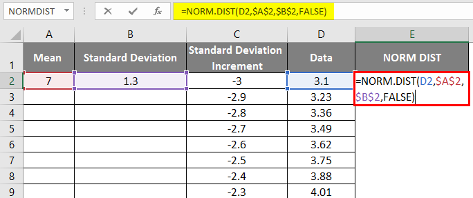
- We will get the below result as follows.
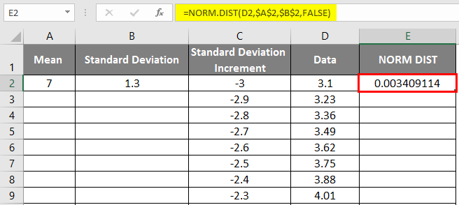
- Drag the values to get the exact result which is shown below.
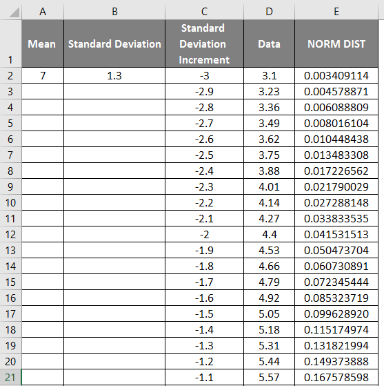
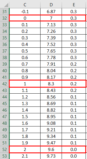
- As shown in the above screenshot, we calculated the NORMAL distribution from the mean and standard deviation. Now let’s see what will be the inverse of NORMAL distribution by applying the NORMSINV, which is shown below.
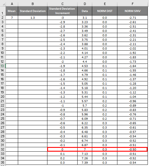
- Here, Value Zero (0) has a standard deviation of 7.
![]()
Applying scattered graph to look at how the left and right curve appears.
- First, select the data and the Normal column.
- Go to the Insert tab and select the scattered graph as follows.
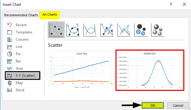
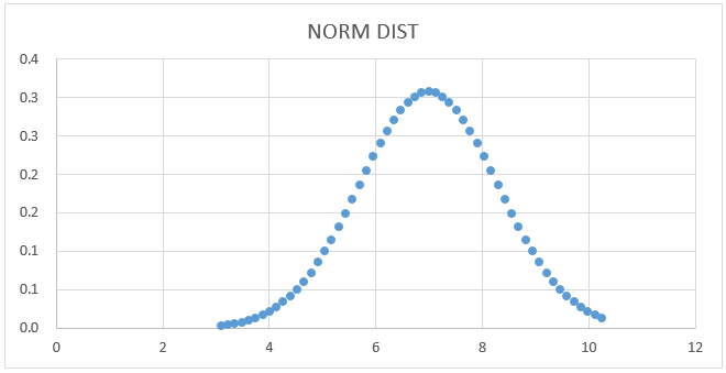
- We will get the below curve graph as shown below.
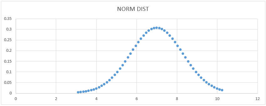
Here we can see that Mean value 7 has a standard deviation shape, and we can show that by drawing a straight line to represent it.
- Mean =7
- 1 –Standard deviation indicates 68% of Data.
- 2 –Standard deviation indicates 95% of Data.
- 3 –Standard deviation indicates 99.7% of Data.
Normal Distribution Graph:
NORMSINV Graph:
Select the data column and NORM SINV from the above figure to get the graph below.
- First, select the data and the Normal column.
- Go to the Insert tab and select the scattered graph.
- We will get the below graph which is shown in the below screenshot.
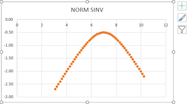
- From the above screenshot, we can see that we got an exact inverse of a normal distribution which shows the same value figure below.
![]()
Example #3 – Configuring the Left and Right Curve
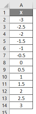
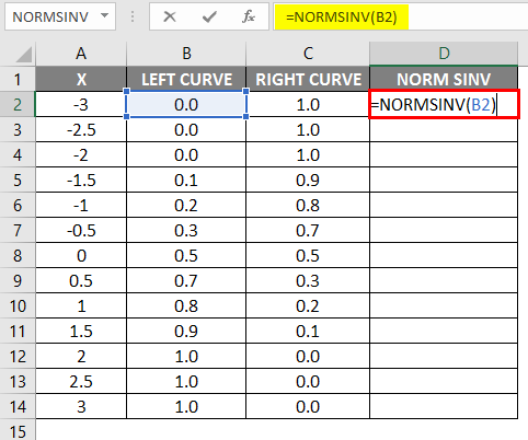
We will configure the left and right curves using the normal distribution function in this example. Consider the data below, where x has negative values and gets incremented to positive values.
- Apply the formula =NORM.DIST(A2,0,1,1).
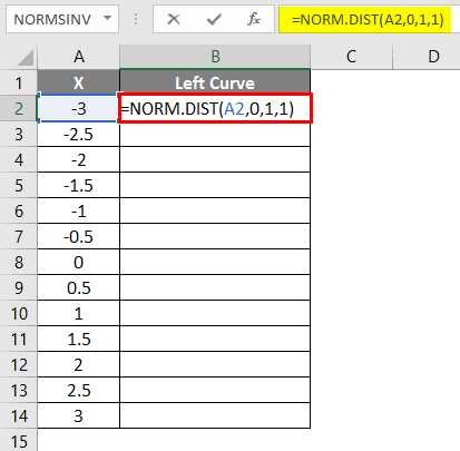
- After applying the formula, the result is shown below.
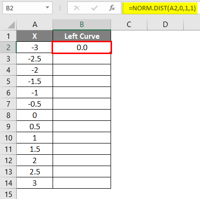
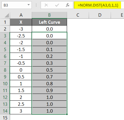
- Drag the formula into other cells.
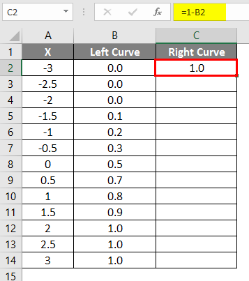
- Apply formula =1-B2.
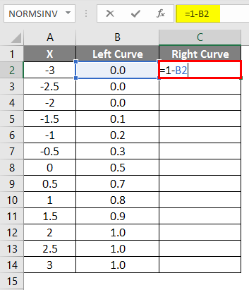
- After applying the formula, the result is shown below.
- Drag the same formula into other cells.
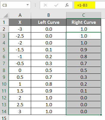
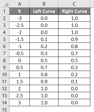
The result of the above-applied formula is shown below.
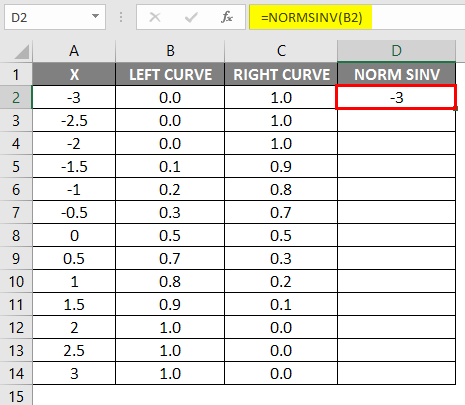
- Left curve values have been calculated by applying the NORMAL DISTRIBUTION formula by setting the cumulative value as True, and the NORMSINV has been calculated using the left curve.
- After applying the formula, the result is shown below.
- Drag the same formula into other cells.
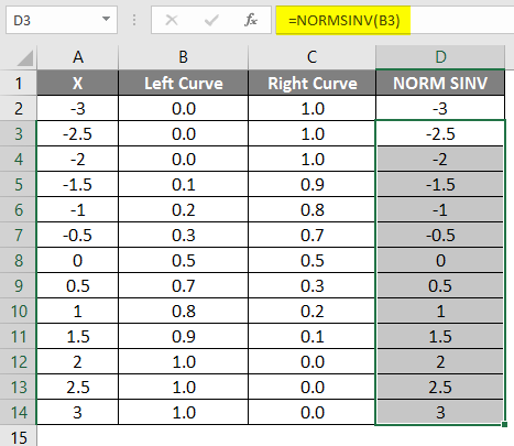
As we can see that we got the same value for NORMSINV, which is nothing but the inverse of the normal distribution. In the same way, we will get the right curve value by calculating the 1-left curve value. In the next step, we will check how we get the x’s height using the scattered graph.
- Select the left cure and right curve columns.
- Go to insert menu.
- Select the scattered graph as follows.

We will get the below graph result as shown below.
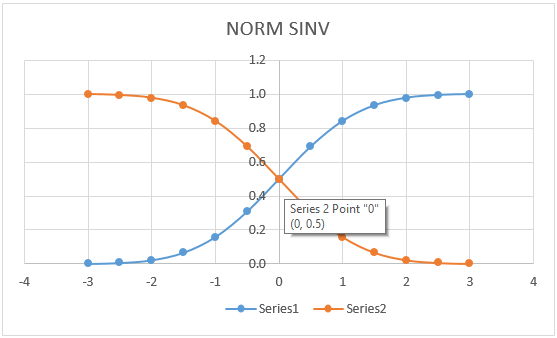
NORM SINV Graph:
The graph below shows that the NORM DISTRIBUTION value left curve has the exact match for (0, 0.5 ), which lies at the center of the line where we will get the same graph if we apply for NORMDIST.
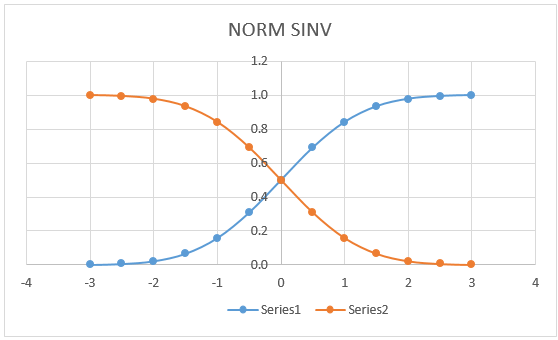
Here in the above graph it shows very clearly that we got the exact mean at a center point which denotes:
- X=0
- Left Curve=0.5
- Right Curve=0.5
We displayed it to view the NORMSINV values in a graphical format, as shown below.
Things to Remember About Excel NORMSINV
- #value! The error occurs when the given argument is a non-numeric or logical value.
- In the Normal Distribution function, we usually get #NUM! Error due to the standard deviation argument is less than or equal to zero.
Recommended Articles
This is a guide to Excel NORMSINV. Here we discuss how to use NORMSINV in Excel, practical examples, and a downloadable Excel template. You can also go through our other suggested articles –
