Updated August 11, 2023
Introduction to Freeze Panes in Excel
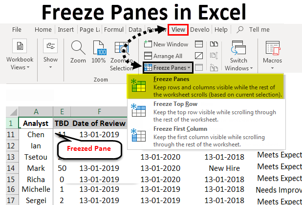
Freeze Panes in Excel are used to fix any frame, row, or section of the table to access the data located below so that the user can also see the header’s name. There is 3 type of Freeze Panes option available in the View menu tab under the Window section, Freeze Panes, Freeze Top Row, and Freeze First Column. Freeze Panes are used to freeze the worksheet from where we keep our cursor. This freezes both the row and column both. Then to freeze a Row and a Column, we have a separate option to freeze each of them. Once we do that, we will see some portion of the worksheet will only move once we unfreeze it.
- A Frozen top row to know which parameters we are looking at during a review:
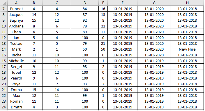
Before Freezing Top Row:
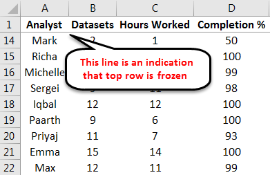
After Freezing Top Row:
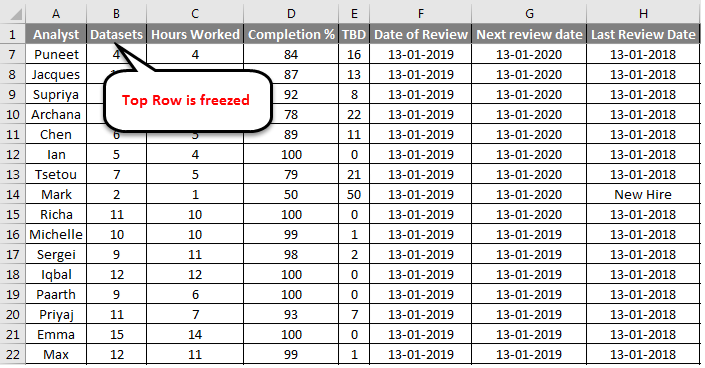
This shows how the same dataset looks with a frozen row. This makes it easy to know which parameter we refer to when analyzing data beyond the first few records in the workbook.
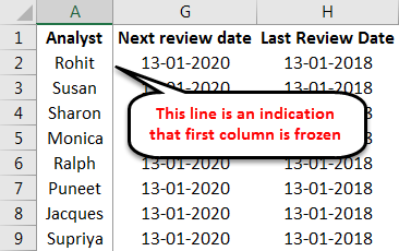
- A frozen first column to know which record we are evaluating for a particular parameter.
Before freezing the first column:
After freezing the first column:
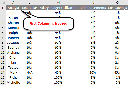
Freezing Panes allows us to split the dataset into multiple parts to ease analysis: The worksheet gets split into different parts, which can be browsed independently. The figure above compares the dataset with and without the first column frozen. The Grey Lines in the middle of the worksheet indicate where the rows and columns have been frozen.
How to Freeze Panes in Excel?
The Freeze Panes feature is not very complicated if we know the database we are working with. In the next few paragraphs, we will learn how to use the features associated with freezing panes and using them for analysis.
Here are a few examples of Freeze Panes in Excel:
Freeze Top Row – Example #1
To do this, we have to perform the following steps:
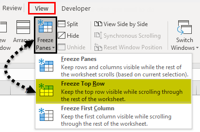
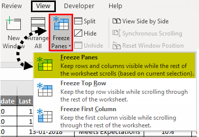
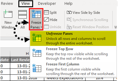
- Select View from the Excel toolbar. Select Freeze Panes from the view options; this will open a dropdown menu with options to select the rows or columns we want to freeze. Select Freeze Top Row; this will keep the active worksheet’s top row in place and allow us to browse the rest of the data without disturbing the top row.
- A Tiny grey straight line will appear just below the 1st row. This means the first row is locked or frozen.
Freeze First Column – Example #2
Next, we look at the next most commonly used function in the Freeze Pane feature, freezing the first column. This can be done using the following steps:
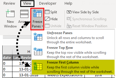
- Select Freeze Panes from the view options. From the dropdown menu, select Freeze First Column, and this would freeze the first column in place, allowing us to browse the rest of the data without disturbing the first column.
A Tiny grey straight line will appear just below the 1st Column. This means the first column is locked or frozen.
These features can be used simultaneously, making it easier for us to analyze data. As we have seen in the examples, knowing the table’s basic structure helps us decide what we want to freeze.
Freeze First Row and First Column – Example #3
Freeze the first row and first column.
Here is an example of the practice table with the frozen first row and first column.
This brings us to the most useful function in the freeze panes feature, freezing multiple columns and rows.
I like to use this function the most because it enables the user to freeze rows and unfreeze rows and columns based on any number of parameters depending on the structure of the worksheet’s data.
To freeze the first row and first column, we need to perform the following steps:
- Select Cell B2 from the worksheet.
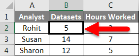
- Now, from the view options, select Freeze Panes. From the dropdown that appears, select the first option, Freeze Panes.
These actions freeze the first row and first column in place.
Freeze Multiple Columns – Example #4
We can use similar steps to freeze multiple rows and columns. The following steps illustrate this:
- Select any cell above which the rows and columns have to stay in place:
- Repeat steps 2 and 3 from the previous illustration to freeze all rows and columns above and left of the selected cell.
The solid grey lines indicate that the rows and columns on the top left of the sheet have been frozen. We can also choose a whole row above which we need data to stay in place or a column.
Unfreezing rows and columns to their default state are very simple. We have to go into the freeze panes dropdown and click on Unfreeze Panes, as shown below.
Freeze panes in Excel are an option that makes it very easy for us to compare data in large datasets. In fact, freezing panes in Excel are so useful that software providers provide additional features based entirely on freezing panes in Excel. One such example is the ability to freeze and unfreeze multiple worksheets and tables simultaneously, which many software vendors provide as a product.
Things to Remember
- Freeze Panes do not work while editing something inside a cell, so care must be exercised while selecting the cell we want as the frozen data boundary; never double click that cell before freezing the data.
- Freeze panes in Excel are a default configuration that can freeze data to the left of the boundary column or above the boundary row, depending on what we choose as a boundary. There are add on available from various software providers to enhance these.
Recommended Articles
This has been a guide to Freeze Panes in Excel. Here we discussed how to freeze panes in Excel and different methods to freeze panes in Excel, along with practical examples and a downloadable Excel template. You can also go through our other suggested articles to learn more –