Updated September 28, 2023
Economic Examples Introduction
You can find economics surrounding you every day, from choosing to buy a breakfast burrito to making a career decision. Economics is not just present in complex government policies but also in the everyday decisions you make.
Today, we will look at various real-life economic examples of economic principles and factors that affect us and the world around us.
Real-World Economic Examples
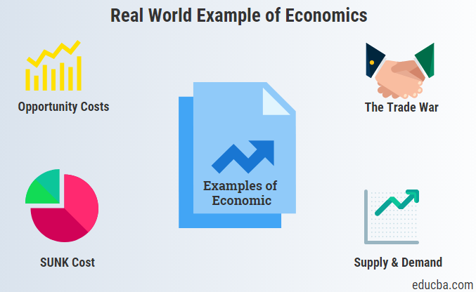
Here are some real-world economic examples related to major economics concepts.
1. Inflation
Inflation is when prices of goods and services keep increasing constantly. This continuous increase in prices reduces the consumers’ purchasing power. For example, the amount of money that lets us buy 100 things today will only let us buy 50 things in the future. So, with the same amount of money, we can’t buy as many things or services as we could before.
Example:
In August 2023, the US experienced a 3.7% increase in prices compared to August 2022. This means that the prices of goods and services, on average, increased by 3.7%. For instance, the prices of food items increased 4.3% in the last 12 months.
2. Trade War
A trade war is an economic conflict between countries. It occurs when countries engage in a series of actions, such as imposing tariffs (taxes) and trade barriers on each other’s goods and services. These actions escalate trade tensions, often leading to a decrease in international trade and causing disruptions in the global economy.
Example:
In 2002, George Bush added 8% to 30% tariffs on imported steel goods to support the struggling American steel industry. This tariff affected 29% of imports, leading the European Union (EU) to file a complaint to the World Trade Organization (WTO). The EU also threatened to put 100% tariffs on American products like fruit juice, T-shirts, etc. However, in December 2003, George Bush removed the tariffs, resolving the trade war.
3. Gross Domestic Product (GDP)
GDP is a metric that countries use to calculate the total value of all goods and services generated within the country during a specific period (year or quarter). When a country’s GDP goes up, it usually means the economy is growing or getting better.
Example:
As of 2022, global GDP exceeded $100 trillion, with the United States leading at $25 trillion, accounting for approximately a quarter of the world’s GDP. China ranked second, followed by Japan and Germany.
4. Supply and Demand
Supply refers to the quantity of a product or service that producers can provide in the market. Demand, on the other hand, represents the quantity of that product or service that consumers want to buy. The interplay between supply and demand sets the price and accessibility of goods and services within an economy.
Example:
Since before 2020, there has been a global shortage of semiconductors. These are important parts useful in creating phones, cars, and medical devices. The shortage was due to the supply and demand mismatch, which resulted from factors like increased demand for semiconductors in various industries, difficulties in getting the required materials, and unexpected events like factory fires and the COVID-19 pandemic. To address this shortage, the private sector is working to increase production, manage supply chains more effectively, and design products that use semiconductors efficiently.
6. Opportunity Costs
Opportunity Cost is the cost of choosing one option over another. It is the value of the option you give up when you allocate your resources (like time, money, or effort) to a particular choice. Essentially, it’s the value of what you could have gained but didn’t because you chose a different path.
Example:
Imagine a company that has some extra money to invest, and they have two options:
- Option 1: Invest in the stock market, which can give them a 15% annual return.
- Option 2: Upgrade their equipment, which will generate a 12% annual return.
Now, if the company chooses Option 2 (upgrading equipment), they miss out on the extra 3% (15% -12%) they could have made with Option 1 (stock market). That 3% they miss out on is called the “opportunity cost.” It’s the profit they give up by choosing one option over the other.
7. Sunk Cost
A sunk cost is the amount of funds/resources that a company/individual has already spent and cannot recover. The concept educates businesses that sunk costs should not influence their future choices or actions. This is because these past expenditures are irrelevant to future decisions.
Example:
A company produces basic cricket bats for $50 and sells them for $90. They are thinking about making better-quality bats, which could cost an extra $20 each. They have already spent money on things like the factory and warehouse, which they can’t get back (sunk costs). So, the decision to make better bats depends mainly on whether they want to spend that extra $20 per bat or not.
Final Thoughts
The above economic examples gave an overview of various economic concepts, including supply and demand, opportunity costs, sunk costs, trade wars, inflation, GDP, and unemployment. While these examples may not include all variants, they provide good economic insight.
Recommended Articles
We hope you learned about various economic factors from this economic examples article. You can also go through our other economics articles to learn more:


