Updated June 27, 2023

Introduction to Decision Tree Types
Decision tree types depend based on the target variable or data mining problem. Here, we will see decision tree types based on the data mining problem. If we see about the decision tree, a decision tree is defined as that given a database D = {t1, t2,….tn} where ti denotes a tuple, which is defined by attributes set A = {A1, A2,…., Am}. Also, given a set of classes C = {c1, c2,…, ck}.
A decision tree is a binary tree that has the following properties:
- First, each internal node of the decision tree is marked with an attribute Ai.
- Second, each edge is labeled with a predicate that can be applied to the attribute associated with the parent node of it.
- Finally, each leaf node is labeled with class cj.
Decision Tree Types in Data Mining
There are two types of decision trees in data mining:
- Classification Decision Tree
- Regression Decision Tree
Here, we will see both decision tree types based on the data mining problems.
1. Classification Decision Tree
A decision tree is a binary tree that recursively splits the dataset until we are left with pure leaf nodes. That means the data is only one type of class. So, for example, there are two kinds of nodes in the classification decision tree: decision nodes and leaf nodes.
The decision node contains a condition to split the data. And the leaf node helps us to decide the class of a new data point. If any child is a pure node, it contains no condition; we don’t need to split this node further. Thus, we can easily classify our data when we get all the leaf nodes of our data set.
How do we split the data set in a classification decision tree?
How our model decides the optimal splits.
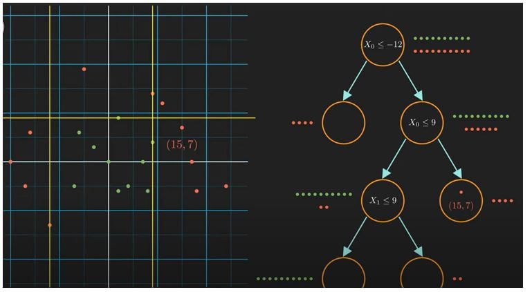
Let’s start at the root.
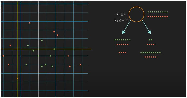
At root, we have the whole data with us. We are going to compare two splits. The first one is x1 <= 4, and the corresponding child nodes look like the first yellow and red dotted lines. The second condition is x0 <= -12, and the corresponding child nodes look like the next yellow and red dotted lines. If you remember, our goal is to get pure leaf nodes; we must go for the second split. Because, in this case, we have successfully produced the left child with red points only. But how can our computers do the same? Well, the answer lies in the information theory. More precisely, our model will choose the split that maximizes the information gain. To calculate information gain, we first need to understand the information contained in a state. Let’s look at the root state; here, the number of red and green points is the same. This means this state has the highest impurity and uncertainty. The way to quantify this is to use entropy.
Where p_i= probability of class i.
We are very uncertain about the randomly picked point if entropy is high. Using this formula, we will calculate the entropy of the remaining four states. The node which has minimum entropy is called a pure node. To find the information gain corresponding to a split, we need to subtract the child nodes’ combined entropy from the parent node’s entropy.
The split, which gives the greater information gain, we will choose that split.
2. Regression Decision Tree
How we solve a regression problem using a decision tree. Well, the basic concept is the same as the decision tree classifier. We recursively split the data using a binary tree until we are left with pure leaf nodes. There are two differences: how we define impurity and make a prediction.
How do we split the data set in a regression decision tree?
It is the most essential part of how we split the dataset.
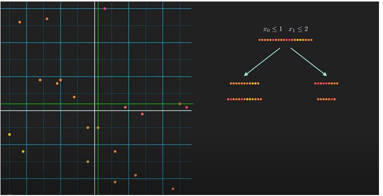
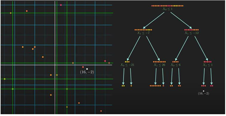
Here, we have the whole dataset, and the task will be to find the best splitting condition. For this, we will examine two candidate conditions; the first condition is x0 is less than or equal to 1; in this case, the split will look like the first dotted lines. And our second condition is x1 less than or equal to 2; in this case, the division is like second dotted lines. Don’t forget the point that satisfies the condition go to the left and the rest to the right. Now, the question is, which is a better split? To find this, we need to calculate which split decreases the impurity of the child nodes the most. For that, we need to compute variance reduction. Yes, we use variance to measure impurity in the context of regression.
Focus on the complete dataset; we are going to compute the variance of the whole dataset using this formula:
Remember, a higher value of variance means a higher impurity. So, first, compute the variance for the root node and then for the divided individual dataset. Then we will compute the variance reduction. For that, we subtract the combined variance of the child nodes from the parent node. The weights are just the relative size of the child concerning the parent. If we compute variance reduction for both the conditions x0 <= 1 and x1 <= 2, we will get that the variance reduction for the first split is much more than the second one. This tells us that the first split can decrease the impurity much more than the second one. So finally we conclude that we should choose the first one.
Conclusion
We can divide the decision tree on both the basis, based on the target variable or the basis of the data mining problem. Their types, how they split the data, and choose the optimal answer for the given condition.
Recommended Articles
We hope that this EDUCBA information on “Decision Tree Types” was beneficial to you. You can view EDUCBA’s recommended articles for more information.
