Updated August 22, 2023
Ctrl Shift-Enter in Excel (Table of Contents)
Excel Ctrl Shift-Enter
Ctrl Shift-Enter is one of the shortcuts used in Excel to perform calculations with array formulae. It supports performing complex calculations using the standard Excel functions. It is widely used in array formulae to apply functions and formulas to a data set. Using Ctrl Shift-Enter together helps convert the data into an array format consisting of multiple data values in Excel. It also supports differentiation between the regular formula and the array formula. This shortcut has two major advantages: dealing with a set of values and returning multiple values at a time.
Explanation of Ctrl Shift-Enter in Excel
- Before we use the shortcut CTRL SHIFT-ENTER, we need to understand more about the arrays. Arrays are data collection, including text and numerical values, in multiple rows and columns or only in a single row and column. For example, Array = {15, 25, -10, 24}.
- To enter the above values into an array, we need to enter CTRL SHIFT+ENTER after selecting the range of cells. It results in the array as Array= {= {15, 25, -10, 24}}.
- As mentioned above, the formula encloses braces around the range of cells, resulting in a single horizontal array. This keyboard shortcut works in different versions of Excel, including 2007, 2010, 2013, and 2016.
- CTRL SHIFT-ENTER also works for vertical and multi-dimensional arrays in Excel. This shortcut works for different functions requiring data in various cells. It is effectively used in various operations like determining sum and performing matrix multiplication.
How to Use Ctrl Shift-Enter in Excel?
CTRL SHIFT-ENTER is used in many applications in Excel.
- Creation of array formula in matrix operations such as multiplication.
- Creation of an array formula in determining the sum of the set of values.
- Replacing the hundreds of formulas with only a single array formula or summing the range of data that meets specific criteria or conditions.
- Counting the number of characters or values in the range of data in Excel.
- Summing the values presented in every nth column or row within low and upper boundaries.
- Performing the task of the creation of simple datasets in a short time.
- Expanding the array formula to multiple cells.
- Determining the Average, Min, Max, Aggregate, and array expressions.
- Returning the results in multiple and single cells by applying the array formulas.
- Use of CTRL SHIFT-ENTER in IF functions.
Examples of Ctrl Shift-Enter in Excel
Below are examples of Excel control shift-enter.
Example #1 – To Determine Sum
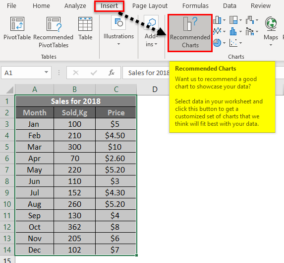
This example illustrates the use of Ctrl SHIFT-ENTER in calculating the sum of sales generated for different products. We consider the following data for this example.
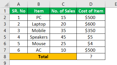
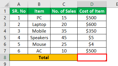
Step 1: Place the cursor in the empty cell where you want to produce the worth of the product’s total sales.
Step 2: Enter the formula as total = sum (D6:D11*E6: E11), as shown in the below image.
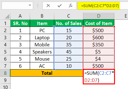
Step 3: After entering the formula, press CTRL SHIFT-ENTER to convert the general formula into an array formula.
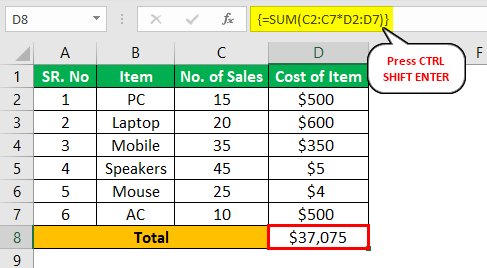
Step 4: The opening and closing braces are added to the sum formula. The result is obtained as shown in the image.
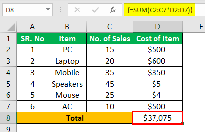
Step 5: Check the result determining the total with the general procedure we used.
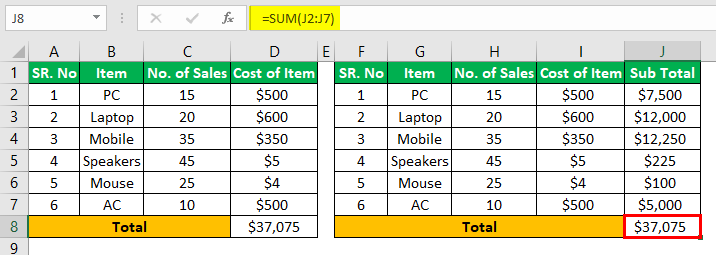
The result obtained from the two procedures is the same. But, using the array formula with CTRL SHIFT ENTER is easy to determine total sales by eliminating the calculation of an additional column of the subtotal.
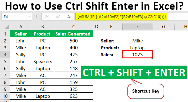
Example #2 – Determine the Sum using Condition
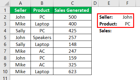
This example illustrates using Ctrl SHIFT-ENTER in calculating the sum of sales generated for different products using the conditions. The following data is considered for this example.
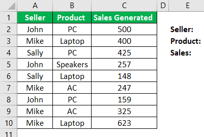
Step 1: In the first step, determine the details of the seller and product that want to calculate sales generated individually. Consider Seller =John and Product = PC and enter these details into respective cells as shown in the below screenshot.
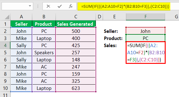
Step 2: To determine the sales generated by John in selling PC products, the formula is
=SUM (IF (((A2:A10=F2)*(B2:B10=F3)), (C2:C10)))
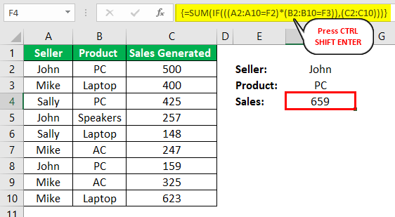
Step 3: Press CTRL SHIFT-ENTER to have the desired result shown in the image.
Step 4: Change the values of F2 and F3 cells to determine sales generated by other persons.
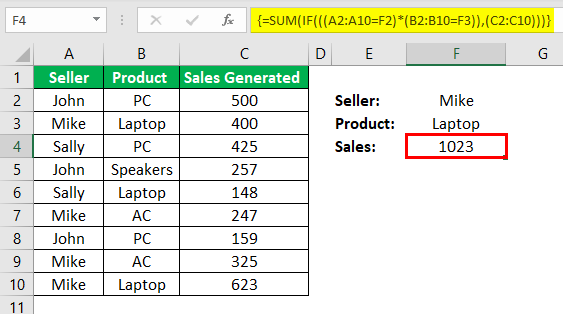
In this way, one can automate the calculation of generated sales by using the shortcut CTRL SHIFT-ENTER.
Example #3 – Determining the Inverse Matrix
For this example, consider the following matrix A.
Let A = 10 8
4 6
Step 1: Enter matrix A into the Excel sheet as shown in the below-mentioned image.
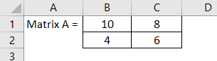
The range of the matrix is B1: C2.
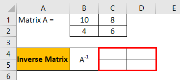
Step 2: Highlight the range of cells to position the inverse matrix A-1 on the same sheet.
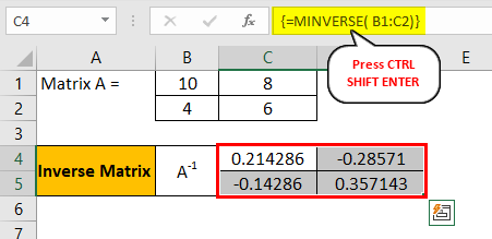
Step 3: After highlighting the range of cells, input the formula of MINVERSE to calculate the inverse matrix. Take care during inputting the formula that all cells are highlighted.
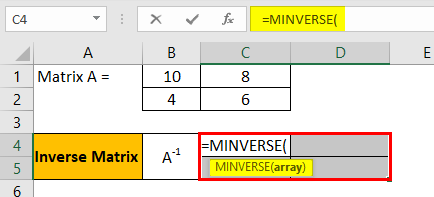
Step 4: Enter the range of the array or matrix as shown in the screenshot.
Step 5: Once the MINVERSE function is entered successfully, use the shortcut CTRL SHIFT-ENTER to generate the array formula to have the results of all four matrix components without reentering to other components. The converted array formula is shown as {=MINVERSE (B1: C2)}
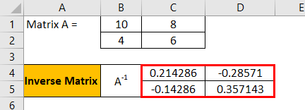
Step 6: The resultant inverse matrix is produced as:
Things to Remember
- Manual entering of braces surrounding the formula doesn’t work in Excel. We should press the shortcut CTRL SHIFT-ENTER.
- When we edit the array formula, we must press the shortcut CTRL SHIFT-ENTER again since the braces are removed every time we make changes.
- While using the shortcut requires selecting the range of cells to result in the output before entering the array formula.
Recommended Articles
This is a guide to CTRL Shift-Enter in Excel. Here we discuss 3 ways to use Ctrl Shift-Enter in Excel to determine the sum, inverse matrix, and sum using condition, examples, and a downloadable Excel template. You may look at our following articles to learn more –
