Updated August 23, 2023
Introduction to COUNTIFS in Excel
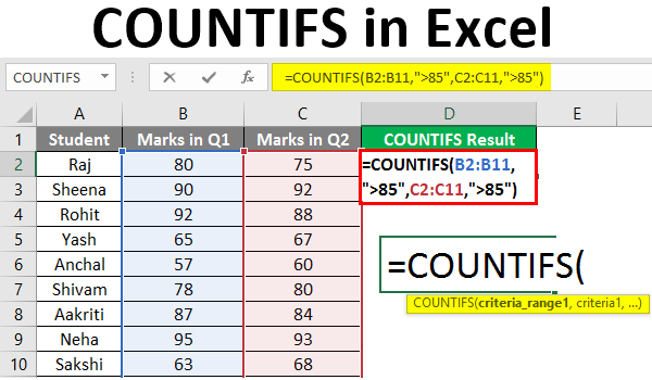
‘COUNTIFS’ is a statistical function in Excel that is used to count cells that meet multiple criteria. The criteria include a date, text, numbers, expression, cell reference, or formula. This function applies the mentioned criteria to cells across multiple ranges and returns the count number of times the criteria are met.
COUNTIFS Function Syntax:
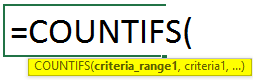
COUNTIFS Function Arguments:
- range1: Required represents the first range of cells we wish to evaluate if it meets the criteria.
- criteria1: Required represents the condition or criteria to be checked/tested against each value of range1.
- range2: Optional represents the second range of cells we wish to evaluate if it meets the criteria.
- criteria2: Required represents the condition or criteria to be checked/tested against each value of range2.
A maximum of 127 pairs of criteria and ranges can enter into the function.
The number of rows and columns of each additional range provided should be the same as the first range. If there is a mismatch in the length of ranges or when the parameter supplied as criteria is a text string greater than 255 characters, then the function returns a #VALUE! Error.
How to Use COUNTIFS in Excel?
Let’s understand how to use COUNTIFS in Excel with a few examples.
Example #1 COUNTIFS Formula with Multiple Criteria
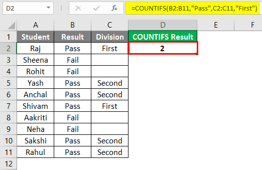
Let’s say we have the result status of a class of students, and we wish to find a count of students who have passed as well as scored ‘First Division’ marks.
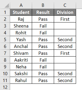
Students ‘Pass/Fail’ status is stored in column B. The result status according to marks, i.e., if it is ‘First Division’ or not, is stored in column C. The following formula tells Excel to return a count of students who has passed and scored ‘First Division’ marks.
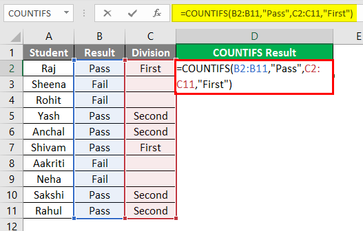
So we can see in the above screenshot that the COUNTIFS formula counts the number of students who meet both conditions/criteria, i.e., who have passed and scored ‘First Division’ marks. The students corresponding to the below-highlighted cells will be counted to give a total count of 2, as they have passed and scored ‘First Division’ marks.
Example #2 COUNTIFS Formula with the Same Criteria
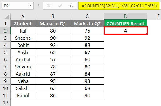
Let’s say we have scores/marks of a class of students in the first two quarters, and we wish to find the count of students who scored more than 85 in both quarters. The scores of students in Quarter 1 are stored in column B, and those in Quarter 2 are stored in column C. Then, the following formula tells Excel to return a count of students who scored more than 85 marks in both quarters.
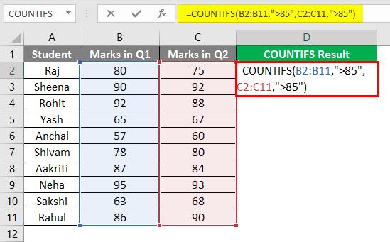
So we can see in the above screenshot that the COUNTIFS formula counts the number of students who have scored more than 85 marks in both quarters. Students corresponding to the below-highlighted cells will be counted.
Example #3 Count Cells whose Value lie between Two Numbers
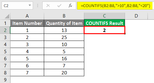
Let’s say we have two columns containing item numbers and their quantities present in a store. If we wish to find out the count of those cells or items whose quantity is between 10 and 20 (not including 10 and 20), we can use the COUNTIFS function below.
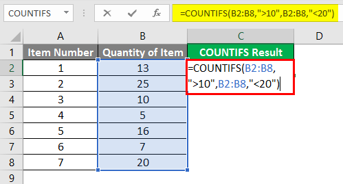
So we can see in the above screenshot that the formula counts those cells or items whose quantity is between 10 and 20. Items corresponding to the below-highlighted values will be counted to give a total count of 2.
Example #4 Criteria is a Cell Reference
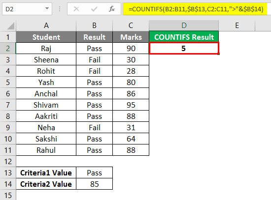
Let’s say we have the result status (Pass/Fail) of a class of students and their final marks in a subject. Now, if we wish to find a count of those students who have passed and scored more than 85 marks, then, in this case, we use the formula as shown in the screenshot below.
So we can see in the above screenshot that cell reference is passed in the criteria rather than supplying direct value. Concatenate (‘&’) operator is used between the ‘>’ operator and the cell reference address.
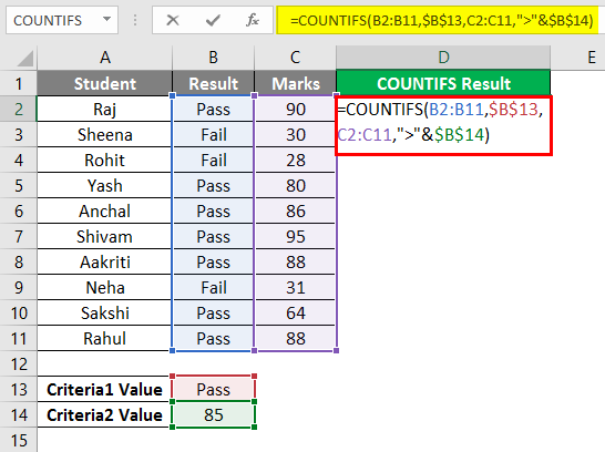
The students corresponding to the below-highlighted cells will be counted to give a total count of 5, as they meet both conditions.
Things to Remember About COUNTIFS in Excel
- COUNTIFS is useful in cases where we wish to apply different criteria on one or more ranges. In contrast, COUNTIF is useful in cases where we wish to apply a single criterion to one range.
- We can use the wildcards in criteria associated with the COUNTIFS function: ‘?’ to match a single character and ‘*’ to match the sequence of characters.
- If we wish to find an actual or literal asterisk, question mark, or asterisk in the range supplied, we can use a tilde (~) in front of these wildcards ( ~*, ~?).
- If the argument provided as ‘criteria’ to the COUNTIFS function is non-numeric, it must be enclosed in double quotes.
- The COUNTIFS function only counts cells that meet all the specified conditions.
- Both contiguous and non-contiguous ranges are allowed in the function.
- We should try to use absolute cell references in criteria and range parameters to avoid breaking the formula when copied to other cells.
- COUNTIFS can also be used as a worksheet function in Excel. The COUNTIFS function returns a numeric value. COUNTIFS function is not case sensitive in the case of text criteria.
- If the argument provided as ‘criteria’ to the function is a blank cell, then the function treats it like a zero value.
- The relational operators that can be used in expression criteria are:
- Less than operator: ‘<.’
- Greater than operator: ‘>.’
- Less than or Equal to the operator: ‘<=.’
- Greater than or Equal to an operator: ‘>=.’
- Equal to the operator: ‘=.’
- Not Equal to the operator: ‘<>.’
- Concatenate operator: ‘&’
Recommended Articles
This is a guide to COUNTIFS in Excel. Here we discuss how to use COUNTIFS in Excel, practical examples, and a downloadable Excel template. You can also go through our other suggested articles –
