Updated August 19, 2023
Compare Two Columns in Excel
Compare Two Columns in Excel comparing the values in those columns. There are different ways to do this. In the first way, we can select the parallel cells of the columns, which we want to compare by separating them with an equal sign (“=”). This will give us the output as TRUE and FALSE. If a cell of the columns is matched, we will get TRUE, else FALSE. In another way, we can use the IF function to match the column cells the way we do by putting an equal sign to get the message we want when columns are matched.
How to Compare Two-Column Data? Top Methods
There are a lot of ways to do that. They are:
- Compare data in columns – Row-Wise
- Compare two columns Row-wise – Using Conditional Formatting.
- Compare data Column wise – Highlight the matching data
Compare Two Column Data By Row-wise – Methods #1
When we are looking for an exact match, use this technique. Let’s take the below example to understand this process.
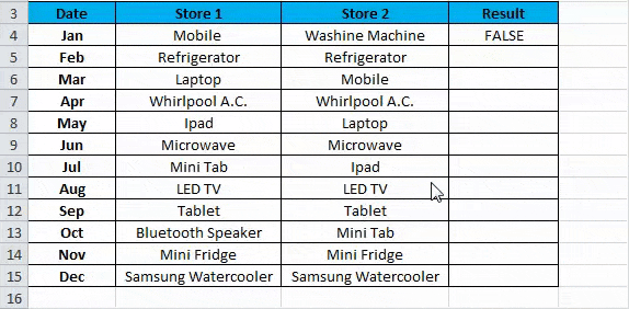
We have given the below dataset where we need to analyze the sold product of two stores month-wise. This means does the customer purchase the same product in the same month?
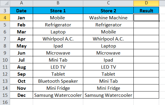
If the same product is being sold month-wise, the result should return as ‘TRUE’; otherwise, ‘FALSE’.
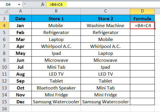
For this, we will apply the below formula:
=B4=C4
Refer to the below screenshot:
The result is shown below:
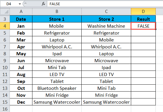
Drag & drop this formula for the rest values, and the result is shown below:
Using Conditional Formatting – Methods #2
By using conditional formatting, we can highlight the data in cells. If the same data point exists row-wise in both columns, we want to highlight those cells. Let’s take an example of this.
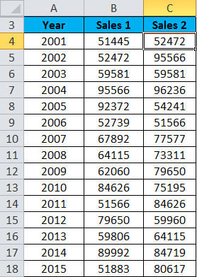
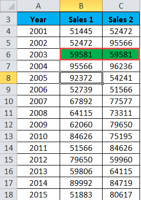
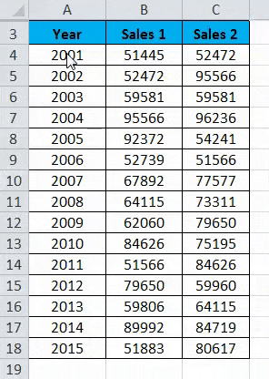
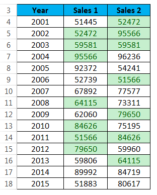
We have given year-wise performance data where we want to analyze if we have achieved the same performance in the same year.
Follow the below steps:
- Select the whole data set range. Here we have selected cell range B4: C18.
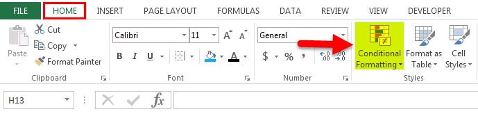
- Go to the HOME tab and click Conditional Formatting under the Styles section. Refer to the below screenshot.
- It will open a drop-down list of formatting options.
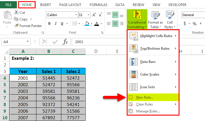
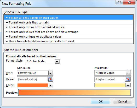
- It will open a dialog box for New Formatting Rule, as shown in the below screenshot. Click on the New Rule option here. Refer to the below screenshot.
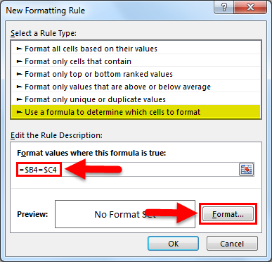
- Click on the last option, “Use a Formula to determine which cells to format“, under the Select a Rule Type section. After clicking on this option, it will display a Formula field, as shown in the below screenshot. Set a formula under the Formula field. The formula we have used here is =$B4=$C4.Click on the Format button to display the Format Cells window.
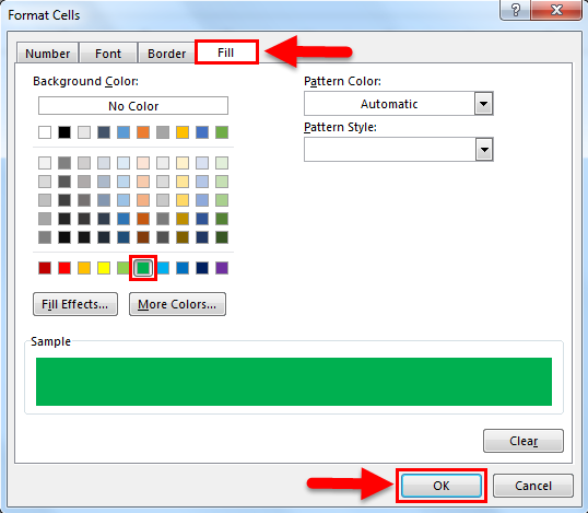
- Click on the Fill tab and choose the color from the color palette. Click on OK. Refer to the below screenshot.
The result is shown below:
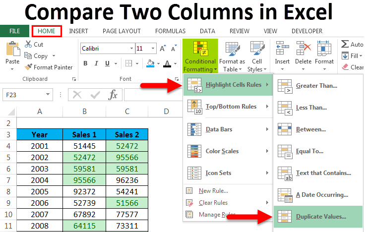
Highlight the Matching data – Methods#3
Here we are comparing the data in the whole list column-wise. Let’s take the below example to understand this process.

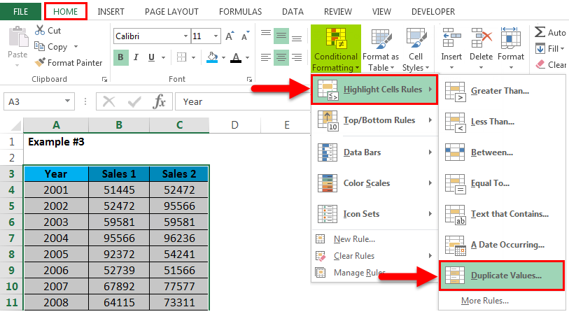
- Select the entire dataset.
- Go to the HOME tab. Click on Conditional formatting under the Styles section. Click on Highlight Cells Rules, and it will again open a list of options. Now click on Duplicate Values from the list. Refer to the below screenshot.
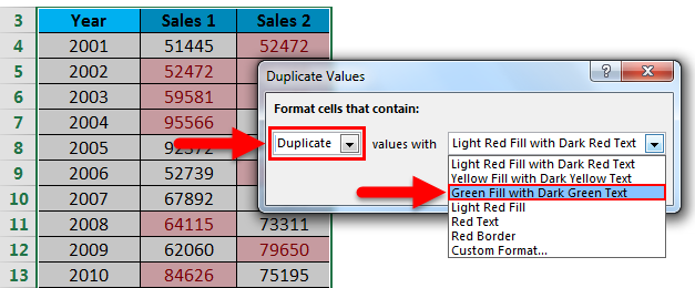
- It will open a dialog box for Duplicate Values. Click for a Duplicate option in the left side field and choose the color for highlighting the cells. Refer to the below screenshot. Click on OK.
- The result is shown below:
Things to Remember about Compare Two Columns in Excel
- We also can highlight the data for the unique values.
- Through these techniques, we can easily compare the data in the dataset and highlight those cells.
Recommended Articles
This is a guide to Compare Two Columns in Excel. Here we discuss Compare Two Columns in Excel and how to use the Compare Two Columns in Excel, practical examples, and a downloadable Excel template. You can also go through our other suggested articles –
