Updated August 21, 2023
Borders in Excel
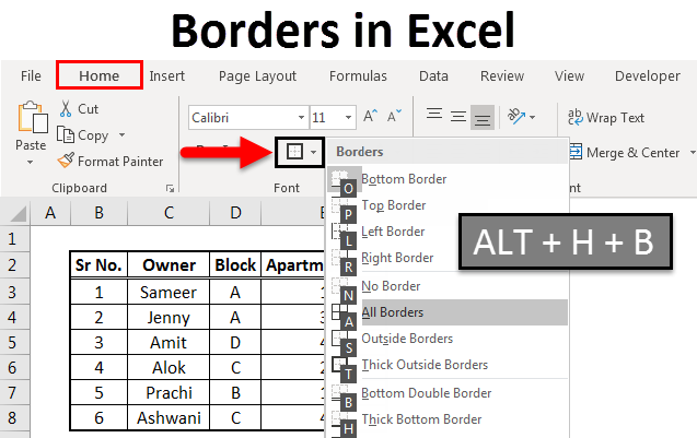
Borders are the boxes formed by lines in the cell in Excel. To distinguish specific values, outline summarized values, or separate data in ranges of cells; you can add a border around cells. By keeping borders, we can frame data and provide them with a defined limit.
How to Add Borders in Excel?
Adding borders in Excel is very easy and useful for outlining or separating specific data or highlighting some values in a worksheet. Normally, we can easily add all top, bottom, left, or right borders for selected cells in Excel. Option for Borders is available in the Home menu, under the font section with the Borders icon. We can also use shortcuts to apply borders in Excel.
Let’s understand how to add Borders in Excel.
Example #1
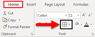
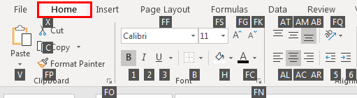
For accessing Borders, go to Home and select the option shown in the screenshot below under the Font section.
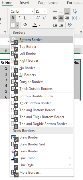
Once we click on the option of Borders shown above, we will have a list of all kinds of borders provided by Microsoft in its drop-down option, as shown below.
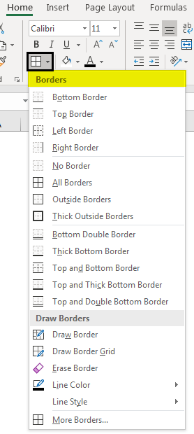
Here we have categorized Borders into 4 sections. This would be easy to understand because all sections are different.
The first is a basic section with only Bottom, Top, Left, and Right Borders. By this, we can create only one side border for one cell or multiple cells.
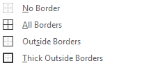
The second section is the full border section, which has No Border, All Borders, Outside Borders, and Thick Box Borders. By this, we can create a full border that can cover a cell and a table. Click No Border to remove the border from the selected cell or table.
The third section combines the bottom borders, Bottom Double Border, Thick Bottom Border, Top and Bottom Border, Top, Thick Bottom Border, and Top Double Bottom Border.
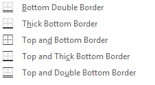
These double borders are majorly used in underlining headlines or important texts.
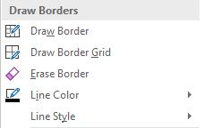
The Fourth section has a customized border section, where we can draw or create a border as needed or change the existing border type. We can also change the border’s color and thickness as well in this section of Borders.
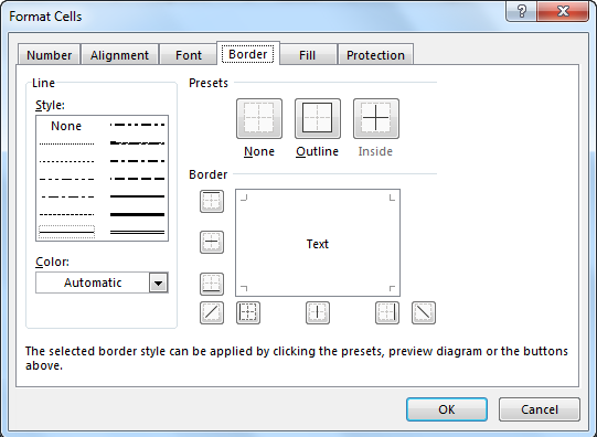
Once we click on the More Borders Option at the bottom, we will see a new dialog box named Format Cells, a more advanced option for creating Borders. It is shown below.
Example #2
We have seen the basic function and use for all kinds of borders and how to create those in the previous example. Now we will see an example where we will choose and implement different Borders and see how those Borders in any table or data can be framed.
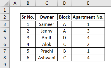
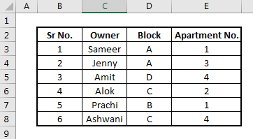
We have a data table with details of the Owner, Block, and Apartment No. Now we will frame the Borders and see what the data would look like.
As row 2 is the headline, we prefer a double bottom line selected from the third section.
And all cells will cover with a box of All Borders, which can select from the second section.
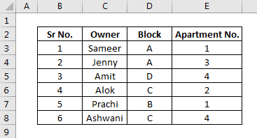
And if we select Thick Border from the second section, the whole table will be bound to a perfect box, and selected data will automatically get highlighted. Once we are done with all the mentioned border types, our table will be like this, as shown below.
As we can see, the complete data table is getting highlighted and ready to be presented in any form.
Example #3
There is another way to frame borders in Excel. This is one of the shortcuts to accessing the functions available in Excel. For accessing borders, the shortcut selects the data we want to frame with borders and then simultaneously presses ALT + H + B to enable the border menu in Excel.

ALT + H will enable the Home menu, and B will enable the borders.

Once we do that, we will get a list of all kinds of borders available in Excel. And this list itself will have the specific keys mentioned to set for any border, as shown and circled in the below screenshot.
After selecting the data table, let’s use All Borders for this case by pressing ALT+H+B+A simultaneously. We can navigate to our required Border type by pressing the Key highlighted in the above screenshot, or we can use direction keys to scroll up and down to get the desired border frame. Once we do that, we will see the selected data is framed with all borders. And each cell will now have its own border in black lines, as shown.
Let’s frame one more border of another type with the same process. Select the data first and then press ALT+H+B+T keys simultaneously. We will see that data is framed with Thick Borders, as shown in the below screenshot.
Pros of Print Borders in Excel
- Creating the border around the desired data table makes data presentable to anyone.
- A border frame in any data set is useful when printing or pasting the data into any other file. By this, we make the data look perfectly covered.
Things to Remember
- Borders can be used with the shortcut Alt + H + B, which will directly take us to the Border option.
- Giving a border in any data table is very important. We must provide the border after every work so the data set can be bound.
- Always align properly so that once we frame the data with a border and use it in different sources, the column width will be automatically set.
Recommended Articles
This has been a guide to Borders in Excel. Here we discussed how to add Borders in Excel and use shortcuts for borders in Excel, along with practical examples and a downloadable Excel template. You can also go through our other suggested articles –
