Updated May 15, 2023
AutoFilter in Excel
IAutofilter in Excel allows us to filter the data on various criteria but not limited to Equal to, Greater than, Greater than or equal to, Contains, and Does not contain. And there are 2 ways to enable this. First is pressing the shortcut keys Shift + Ctrl + L together and choosing the relevant filter criteria from the drop-down menu list. And another is by enabling the filter from the Data menu tab and then selecting the appropriate criteria from that dropdown.
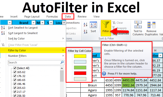
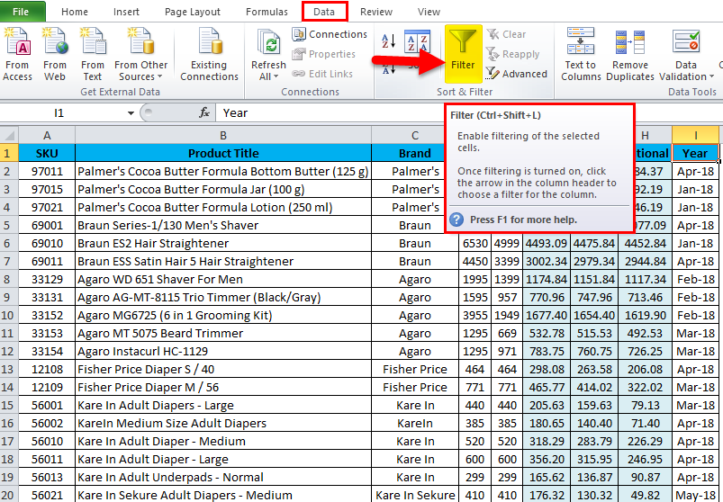
In Excel, we can find the Autofilter option in the data tab in the sort and filter group; click filter as shown in the below screenshot:
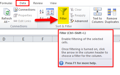
The shortcut key for applying a filter is CTRL+SHIFT+ L, which applies a filter for the entire spreadsheet.
How to Use AutoFilter in Excel?
AutoFilter in Excel is very simple and easy to use. Let’s understand the working of Excel AutoFilter by some examples.
AutoFilter in Excel – Example #1
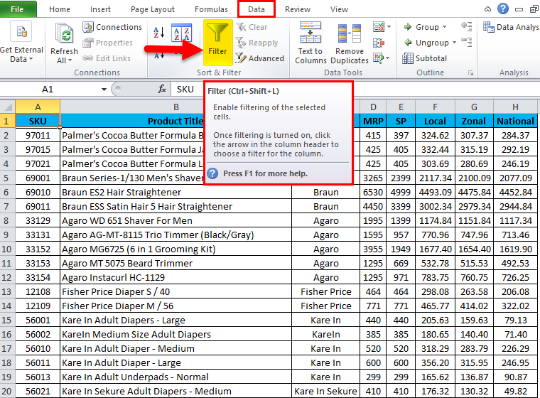
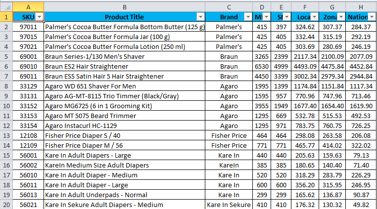
Consider the below example where we have BRAND sales data like local, zonal, and national wise.
We must filter only the specific brand sales to view the sales data. In this scenario, filters can use, which will be very useful for displaying only the specific data. Now let’s see how to apply the Excel Autofilter by following the below procedure.
- First, select the cell to apply a filter. Go to Data Tab. Choose the Autofilter option.
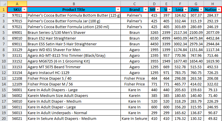
- We can see that a filter has been applied for the entire cells.
- Now we need to filter the specific brand to check the sales.
- We can find BRAND in the C column; click on the drop-down list where it shows all the brands as per the below screenshot.
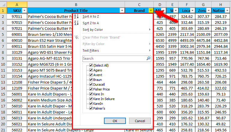
- Unselect all the check marks and select the brand BRAUN from the following list.
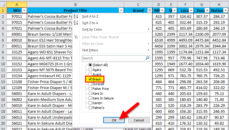
- Once we select BRAUN from the following list, excel filters only BRAUN, and it will hide all the other rows and display the specific brand as the following output.
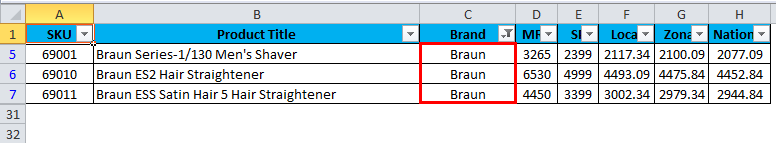
- The above screenshot shows that only brand sales of BRAUN like local, zone, and National wise.
Clear AutoFilter in Excel
- Once the Excel Autofilter has been applied, we can clear the filter where Autofilter has a clear filter option to remove it, shown in the screenshot below.
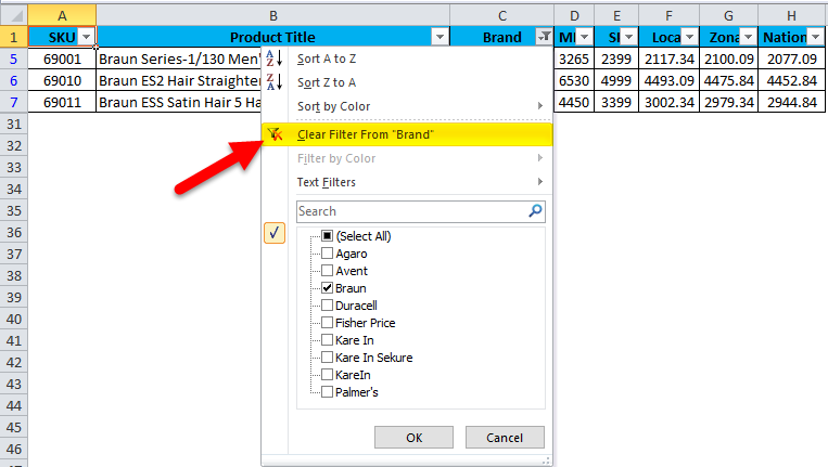
- The above screenshot shows the option “Clear Filter from BRAND” Click on it so that the filters will be removed from the entire spreadsheet.
AutoFilter in Excel – Example #2
In this example, we will now check the year-wise sales and brand wise sales and consider the below example.
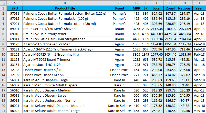
The above screenshot shows the year-wise sales data that has happened for all the brands; let us consider that we need to check the year-wise sales, so by using the filter option, we can do this task to display it.
- Select the cells to apply the filter.
- Go to the Data tab and click the filter option.
- Now the filter has been applied as follows. We can see that the filter has been applied to the entire cell.
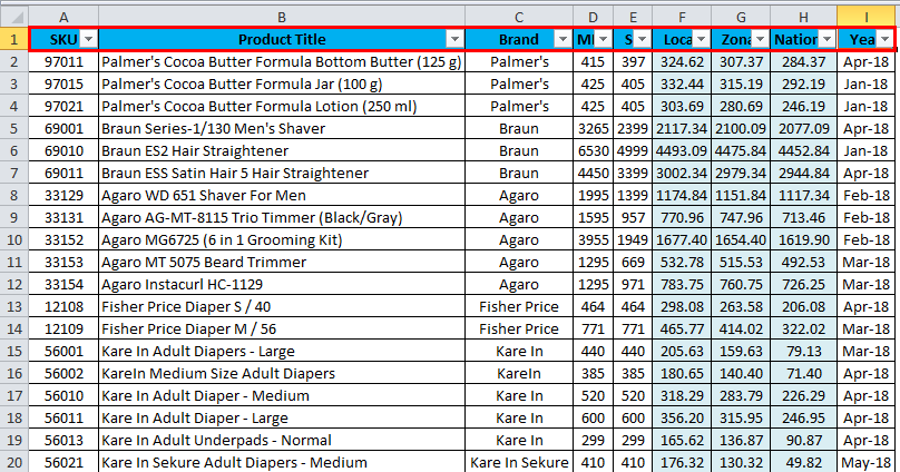
- Select the Year column and click on the drop-down list, and the output is as follows.
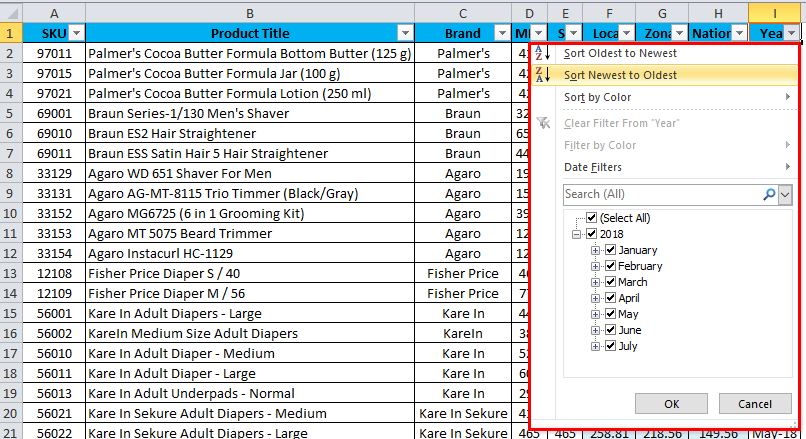
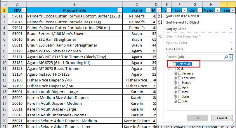
- Once we click on the drop-down list, we can see the month name that has been checked; now, we go to the specific month we need to check for the sales data. Assume that we need to check for April month sales. So remove the select all checkboxes from the list as shown below.
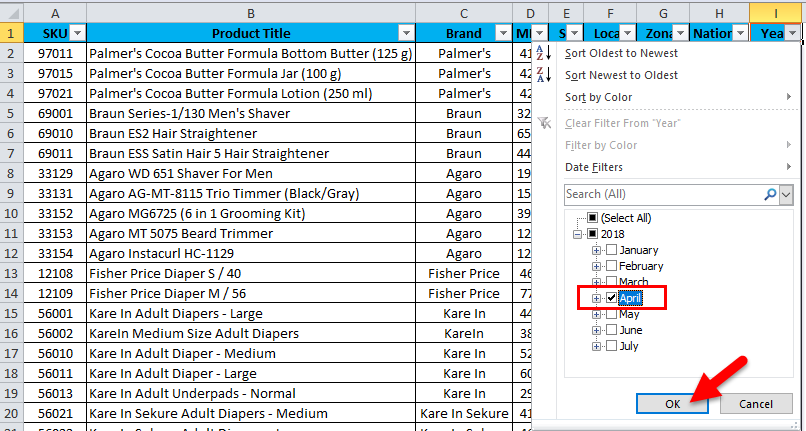
- Now we can see that all checkbox is unselected, and now choose the “APRIL” month to filter only the “APRIL” month sales.
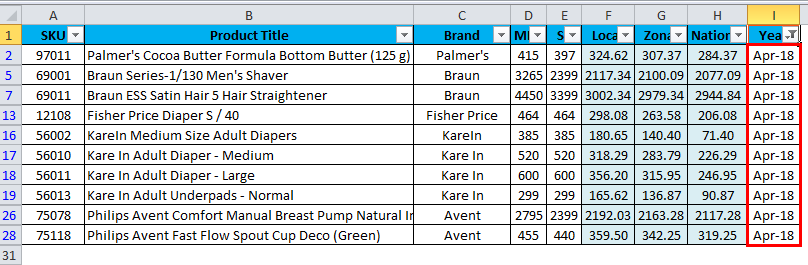
- Here the April sale has been displayed along with brand wise and Local, Zone, and National wise sales. Hence we can give the month-wise sales data by applying the filter option.
AutoFilter in Excel – Example #3
In this example, we will see the number filter, which has various filters.
Let’s consider the same sales data assuming we need to find the zone-wise with the highest sales numbers.
- Select the F column cell named Local.
- Click on the drop-down box to get various number filters as equal, does not equal, greater than, etc.
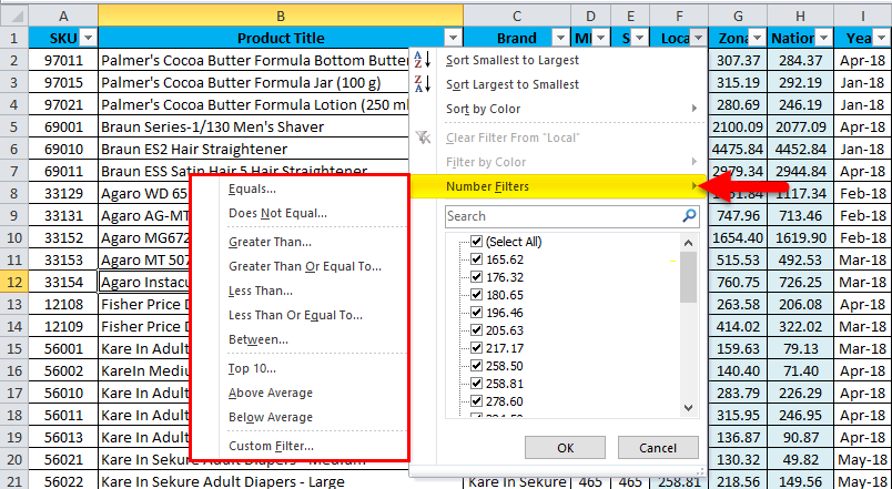
- At the bottom, we can see the custom filter, where we can apply a filter of our choice.
- Click on the custom filter.
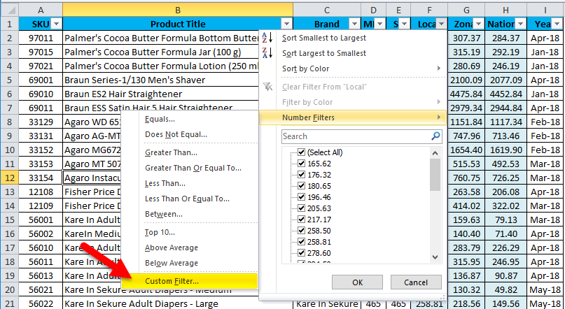
- After choosing the custom filter, we will get a custom dialogue box as follows.
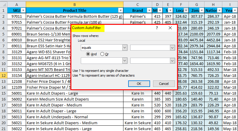
- Click on the custom Autofilter drop-down to get the following list.
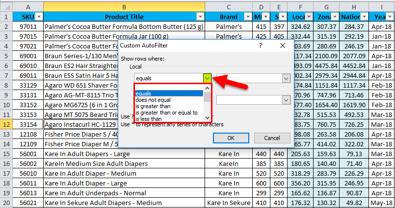
- Choose the “is greater than” option and give the corresponding highest sales values to be get displayed.
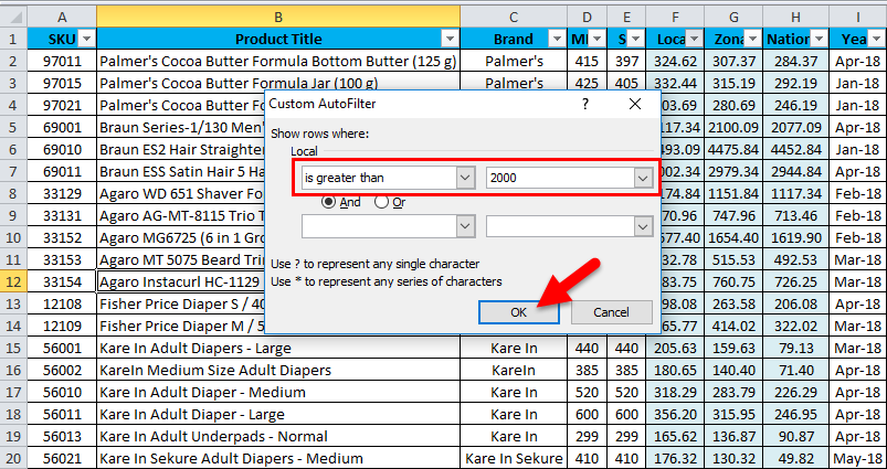
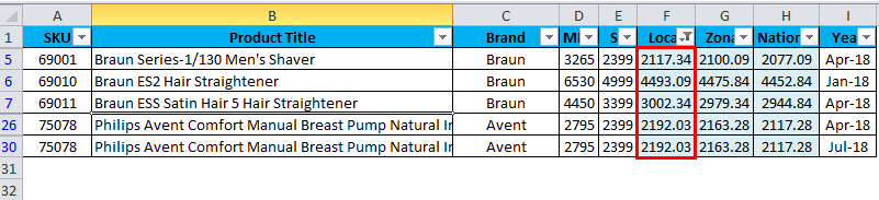
- In the above screenshot, we have given the sales value “is greater than 2000”, So the filter option will display the sales data that has the highest sales value of more than 2000, and the output is displayed as follows.
AutoFilter in Excel – Example #4
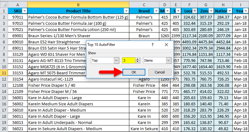
In this example, we will see how to get the top 3 highest sales that have happened for this year.
Consider the same sales data; we can get the top 5 highest sales figures by choosing the Top 10 options given in the number filter as shown below:
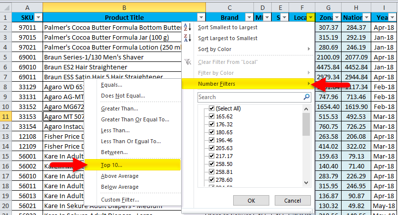
- Click on the top 10 option shown above, and we will get the dialogue box as follows.
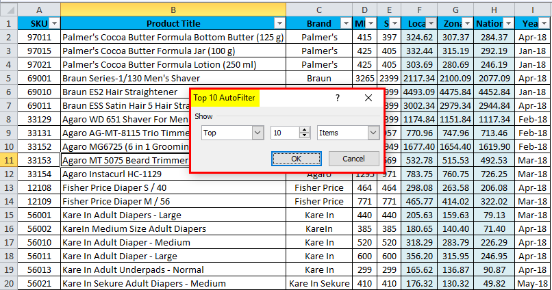
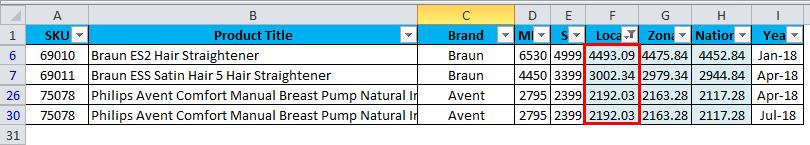
- Here we can increase or decrease the top option numbers as per our choice; in this example, we will consider the top 3 highest sales and then click ok.
- The result below shows the top 3 sales that have happened this year.
AutoFilter in Excel – Example #5
In this example, we will see how to apply a filter by using color, and Normally, in the FMCG field, low sales data values have been highlighted as RED, Medium as Yellow, and Highest Values AS Green. Let us apply the same color for the values and check with the following example.
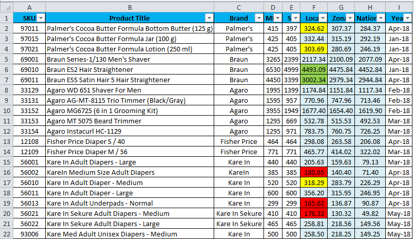
In the above screenshot, we have applied three colors: Red Indicates the Lowest, yellow indicates the Medium, and Green Indicates the Highest Sales value.
- Select the cell F column named Local.
- Click on the drop-down box and select “Filter by Color”.
- Now it shows five different color choices for selection.
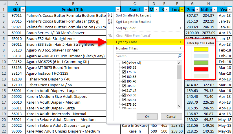
- First, we will select Green to check the highest sales value.

- The output will be as follow.
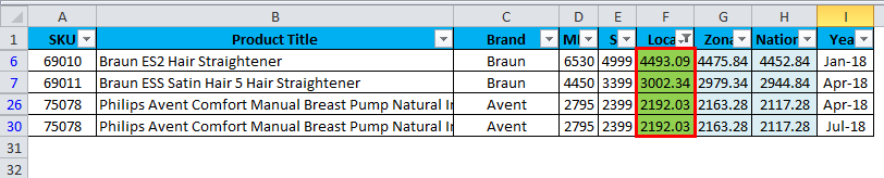
The above result shows that the filter by color has been applied, which shows the highest sale value.
Things to Remember
- Ensure your data is clear and accurate so that we can Autofilter the data easily.
- Ensure to name all the headers before applying AutoFilter, as Excel AutoFilters will not work if the header is blank.
- Before applying the filter, unmerge any cells since Excel Autofilters will not work on merged cells.
- Do not use blank rows and columns while using the Excel AutoFilter.
Recommended Articles
This has been a guide to AutoFilter in Excel. Here we discuss how to use AutoFilter in Excel, practical examples, and a downloadable Excel template. You can also go through our other suggested articles –
