Introduction to Trapezoidal Rule Matlab
Trapezoidal rule is used in integration to compute the definite integral of the functions. It is used extensively in the process of numerical analysis. For the purpose of integration, trapezoidal rule considers the area under curve to be made up of small trapezoids and then calculates the total area by summing the area of all these small trapezoids. In MATLAB, we use ‘trapz function’ to get the integration of a function using trapezoidal rule.
Let us now understand the syntax of trapz function in Matlab:
Syntax:
I = trapz (X)
I = trapz (Y, X)
Description:
- I = trapz (X) is used to calculate the integral of X, using trapezoidal rule. For vectors, it will give approximate integral. For a matrix, it will provide integration over all columns and will return the integration values in a row vector
- I = trapz (Y, X) will integrate X w.r.t coordinates given by Y
Examples of Trapezoidal Rule Matlab
Let us now understand the code to calculate the integration in MATLAB using ‘trapezoidal rule’.
Example #1
In this example, we will take an array representing the (x^2 + 2) and will integrate it using trapezoidal rule. We will follow the following 2 steps:
- Create the input array
- Pass the function to the trapz function
Syntax:
X = [3 6 11 18 27]
I = trapz (X)
Input:
X = [3 6 11 18 27]
I = trapz (X)
Output:
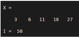
As we can see in the output, we have obtained integration of our input function as 50, which is the same as expected by us.
Example #2
In this example, we will take a function of sin and will integrate it using the trapezoidal rule. We will follow the following 3 steps:
- Define the limits for input sin function
- Create a sin function
- Pass the input function and required limits to the trapz function
Syntax:
Y = 0:100;

X = 10 - 10 * sin (pi / 200 * Y);

I = trapz (Y, X)
Input:
Y = 0:100;
X = 10 - 10 * sin (pi / 200 * Y);
I = trapz (Y, X)
Output:
![]()
As we can see in the output, we have obtained integration of our input function as 363.3933, which is the same as expected by us.
Example #3
In this example, we will take a cos function and will integrate it using the trapezoidal rule. We will follow the following 3 steps:
- Define the limits for input cos function
- Create a cos function
- Pass the input function and required limits to the trapz function
Syntax:
Y = 0:100;

X = 20 - 50 * cos (2*pi / 100 * Y);

I = trapz (Y, X)
Input:
Y = 0:100;
X = 20 - 50 * cos (2*pi / 100 * Y);
I = trapz (Y, X)
Output:
![]()
Example #4
In this example, we will take a matrix and will integrate its rows using the trapezoidal rule. We will follow the following 3 steps:
- Create the vector
- Create a matrix containing observations i.e input data
- Pass the vector and matrix to the trapz function
Syntax:
Y = [2 4.5 7 9];
X = [5    8    6     13;

4     7   15    15;

4     5   10.2 18];
I = trapz (Y, X, 2)
Input:
Y = [2 4.5 7 9];

X = [5    8    6     13;

4     7   15    15;

4     5   10.2 18];

I = trapz (Y, X, 2)
Output:
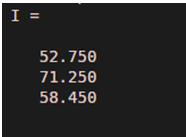
As we can see in the output, we have obtained integration of our input as a column vector, with each element corresponding to one row of the input matrix ‘X’.
Example #5
In this example, we will take a 3×5 matrix and will integrate its rows using the trapezoidal rule. We will follow the following 3 steps:
- Create the vector
- Create a 3×5 matrix containing observations i.e input data
- Pass the vector and matrix to the trapz function
Syntax:
Y = [1 5 8 10 14];
X = [15      8     4     3   0;

12     17    5    11  3;

8      15    10   8   6];
I = trapz (Y, X, 2)
Input:
Y = [1 5 8 10 14];

X = [15      8     4     3   0;

12     17    5    11  3;

8      15    10   8   6];

I = trapz (Y, X, 2)
Output:
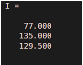
As we can see in the output, we have obtained integration of our input as a column vector, with each element corresponding to one row of the input matrix ‘X’.
Recommended Articles
This is a guide to Trapezoidal Rule Matlab. Here we also discuss the introduction and syntax of trapezoidal rule matlab along with different examples and its code implementation. You may also have a look at the following articles to learn more –
