Updated February 27, 2023

Introduction to Fourier Series Matlab
The following article provides an outline for Fourier Series Matlab. Matlab is a programming environment which is interactive and is used in scientific computing. It is extensively used in a lot of technical fields where problem solving, data analysis, algorithm development and experimentation is required. Software’s which are discipline specific are extensively written using Matlab. Fourier series is used in mathematics to create new functions using sine and cosine waves or functions. The idea of Fourier series was introduced by Baron Fourier. Baron found that we can represent periodic functions by series of sine and cosine waves which are related harmonically to each other.
If a function is periodic and follows below 2 conditions, then the Fourier series for such a function exists.
- f(x) can be absolutely integrated in the range [−π, π] (which implies that Dirichlet integral will be finite).
- f(x) is single valued, piecewise monotonic and piecewise continuous.
Syntax of Fourier Series in Matlab
1. First, we will compute the sine and cos coefficients of Fourier series and also the partial sum of Fourier series. For an expression ‘f’ we can compute ‘nth’ sum in the range / interval [-P, P].
Syntax:
syms z n P x

[initializing the variables]
evalin (symengine, 'assume (z, Type :: Integer)');

[Initializing ‘z’ as an integer variable]
a = @ (f, x, z, P) int (f * cos (z * pi * x / P) / P, x, -P, P);

[Calculating the ‘zth’ Fourier cosine coefficient]
b = @ (f, x, z, P) int (f * sin (z * pi * x / P) / P, x, -P, P);

[Calculating the ‘zth’ Fourier sine coefficient]
fs = @ (f, x, n, P) a (f, x, 0, P) / 2 + ...

symsum (a (f, x, Z, P) * cos (z *pi * x / P) + b (f, x, z, P) * sin (z * pi * x / P), z, 1, n);

[Formula to calculate the nth partial sum]
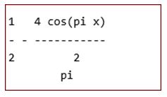
For this example, we will calculate the 2nd partial sum of an absolute function.
f = abs (x)

[absolute function]
pretty (fs (f, x, 2, 1))

[Taking 2nd partial sum; Pretty is used to print x in simple text format]
Code:
syms z n P x

evalin (symengine, 'assume (z, Type :: Integer)');

a = @ (f, x, z, P) int (f * cos (z * pi * x / P) / P, x, -P, P);

b = @ (f, x, z, P) int (f * sin (z * pi * x / P) / P, x, -P, P);

fs = @ (f, x, n, P) a (f, x, 0, P) / 2 + ...

symsum (a (f, x, z, P) * cos (z *pi * x / P) + b (f, x, z, P) * sin (z * pi * x / P), z, 1, n);

f = abs (x)

pretty (fs (f, x, 2, 1))
Output:
2. Next, we will plot the partial sum for n = 4. Our plot will also show the input absolute function.
Syntax:
ezplot (fs (f, x, 4, 1), -1, 1)

[Plotting the 4th partial sum for Fourier series]
hold on

ezplot (f, -1, 1)

[Plotting the absolute function]
hold off

title ('Plotting 4th partial sum')

[Defining the title for the plot]
Code:
ezplot (fs (f, x, 4, 1), -1, 1)

hold on

ezplot (f, -1, 1)

hold off

title ('Plotting 4th partial sum')
Output:
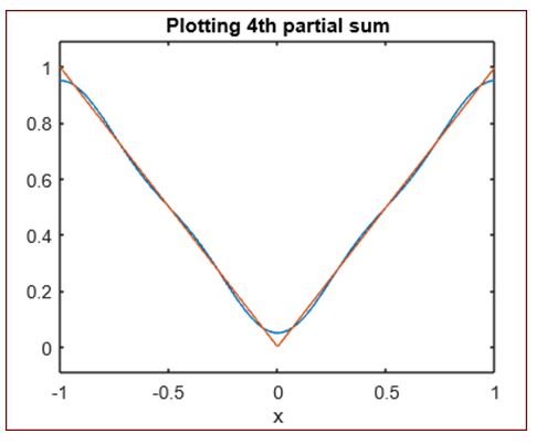
As we can see, we have the plot for our input absolute function and the 4th partial sum of Fourier series.
3. Next, we will plot the 8th partial sum for our Fourier series.
Syntax:
ezplot (fs (f, x, 8, 1), -1, 1)

[Plotting the 8thpartial sum for Fourier series]
hold on

ezplot (f, -1, 1)

[Plotting the absolute function]
hold off

title ('Plotting 8th partial sum')

[Defining the title for the plot]
Code:
ezplot (fs (f, x, 8, 1), -1, 1)

hold on

ezplot (f, -1, 1)

hold off

title ('Plotting 8th partial sum')
Output:
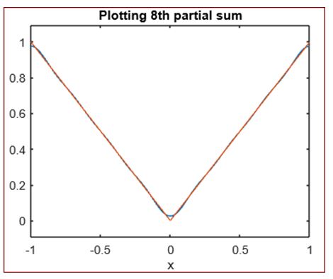
As we can see, we have the plot for our input absolute function and the 8th partial sum of Fourier series.
4. Next, lets take a straight line function as our input and plot its 4th partial sum
Syntax:
syms x z P n

[initializing the variables]
evalin (symengine, 'assume (z, Type :: Integer)');

[Initializing ‘z’ as an integer variable]
a = @ (f, x, z, P) int (f * cos (z * pi * x / P) / P, x,- P, P);

[Calculating the ‘zth’ Fourier cosine coefficient]
b = @ (f, x, z, P) int (f * sin (z * pi * x / P) / P, x, -P, P);

[Calculating the ‘zth’ Fourier sine coefficient]
fs = @ (f, x, n, P) a (f, x, 0, P) / 2 + ...

symsum (a (f, x, z, P) * cos (z * pi * x / P) + b (f, x, z, P) * sin (z * pi * x / P), z, 1, n);

[Formula to calculate the nth partial sum]
f = x

[Input straight line function]
ezplot (fs (f, x, 4, 1), -1, 1)

[Plotting the 4th partial sum for Fourier series]
hold on

ezplot (f, -1, 1)

[Plotting the straight line function]
hold off

title ('Plotting 4thpartial sum')

[Defining the title for the plot]
Code:
syms x z P n

evalin (symengine, 'assume (z, Type :: Integer)');

a = @ (f, x, z, P) int (f * cos (z * pi * x / P) / P, x,- P, P);

b = @ (f, x, z, P) int (f * sin (z * pi * x / P) / P, x, -P, P);

fs = @ (f, x, n, P) a (f, x, 0, P) / 2 + ...

symsum (a (f, x, z, P) * cos (z * pi * x / P) + b (f, x, z, P) * sin (z * pi * x / P), z, 1, n);

f = x

ezplot (fs (f, x, 4, 1), -1, 1)

hold on

ezplot (f, -1, 1)

hold off

title ('Plotting 4thpartial sum')
Output:
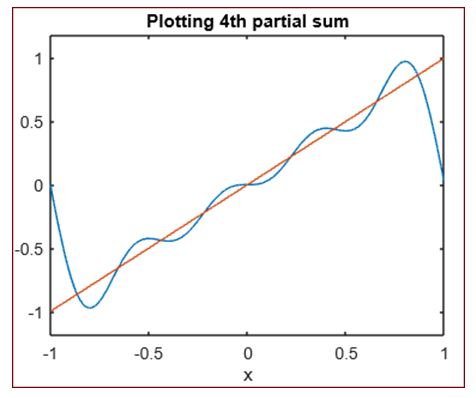
As we can see, we have the plot for our input straight line function and the 4th partial sum of Fourier series.
Conclusion
Fourier series is used in mathematics to create new functions using sine and cosine waves. In Matlab, we can find the Fourier coefficients and plot the partial sums of the Fourier series using the techniques mentioned.
Recommended Articles
This is a guide to Fourier Series Matlab. Here we discuss the introduction to fourier series in matlab, respective syntax with detailed explanation. You may also have a look at the following articles to learn more –
