Updated July 4, 2023
What is SUMIF in Excel?
SUMIF in Excel function provides the sum of values of a certain cell range based on the criteria applied. For example, the formula “=SUMIF(B1:B5, “Pass”, F1:F5)” adds the values (marks) in the cell range F1:F5, which correspond to Pass.
In SUMIF, we can only SUM-specific cells or groups based on one criterion. SUMIF is available under the Formula bar and the Math & Trigonometry bar.

Key Highlights
- We can use SUMIF in Excel to add values with multiple criteria by combining them with the SUMIFS function.
- We can refer to the SUMIFS function as Nested SUMIF, also.
- When we omit sum_range, the SUMIF function in Excel sums up the cells in the particular range.
- We can use wildcard characters such as an asterisk (*) and question (?) marks in criteria related to the text.
- To find a literal question mark or asterisk, we must use a tilde (~) mark in front of the asterisk or question mark in this way— ~* or ~?
- We can use it while doing calculations of a large data table, thus saving time on manual calculations.
- Manual additions can lead to human errors, and SUMIF gives accurate results.
SUMIF in Excel Syntax
range: Cell range(column) in which Excel finds the data that meet the given criteria
criteria: Condition that the selected cell range must follow to perform the calculation
sum_range: Cell range from which values are added based on given criteria.
How to Use the SUMIF in Excel?
To understand the usage of the SUMIF function, let us consider a few examples.
Example #1
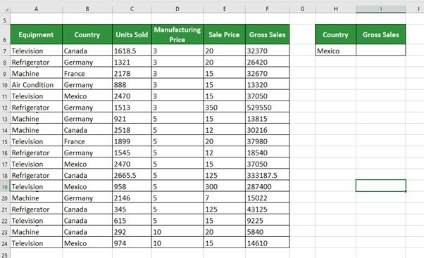
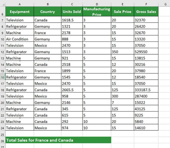
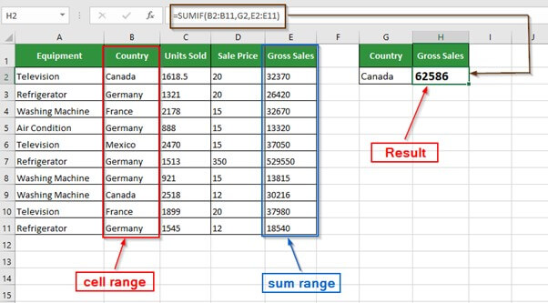
The following table shows a list of branded equipment and their prices. Using the SUMIF function, we need to calculate the total amount spent by the country of Mexico on purchasing televisions.
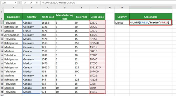
We will apply the SUMIF formula in cell I7 to get Mexico’s total or gross sales.
Step 1: Write =SUMIF and double-click to select SUMIF.
Step 2: Now, select the range B7:B24 and put a comma to separate it from the criteria.
Step 3: Add Mexico in double quotations as the criteria and then put another comma to separate it from the sum column range.
Step 4: Select the range F7:F24 containing the Gross sales amount.
Step 5: Press the Enter key to get the below result.
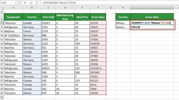
The SUMIF function returns the Gross Sales of 376110 for Mexico.
Example #2
Consider the same data to find the Gross sales of Television for each country.
Step 1: Write the names of all the countries in column H

Step 2: Now, enter the SUMIF formula for the country of Mexico in cell I7 but with a $ symbol, as shown below
=SUMIF($B$7:$B$24,”Mexico”,$F$7:$F$24)

Step 3: Press the Enter key to obtain the Gross Sales for cell I7 (Mexico)
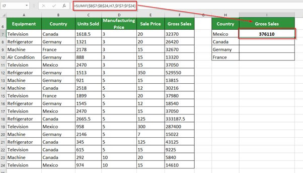
Step 4: Now, copy the formula of cell I7 to cells- I8, I9, and I10 to get the Gross sales for Canada, Germany, and France, as shown in the image below:
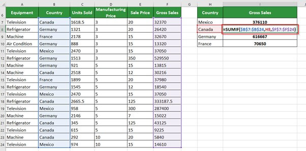
The image above shows that when we put the $ symbol, the range and sum_range remain the same for other cells.
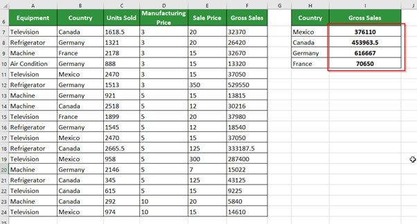
The SUMIF function returns the Gross sales for each country, as shown in the image below:
Example #3
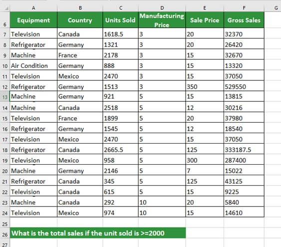
Now, we will find the Total Sale if the unit sold is greater than or equal to 2000 (>=2000)
Step 1: Write Total Sales in cell A26
Step 2: Place the cursor in cell F26 and enter the formula,
=SUMIF(C7:C24,”>=2000″,F7:F24)
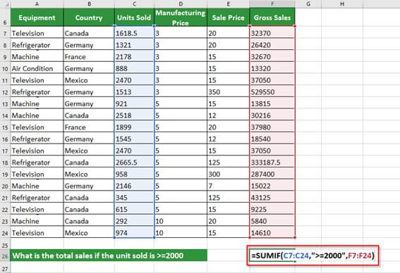
We have used the same logic as in Example #1. Still, instead of selecting the country range and specifying a country name as the criteria, we have chosen the unit sold column as the range and given the criteria as >=2000.
Step 3: Press the Enter key to get the below result
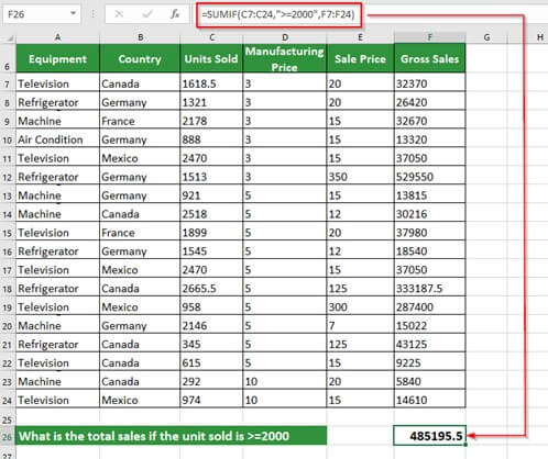
The SUMIF returns the total sales if the unit sold is >=2000 as 485195.5
Example #4
USING WILDCARD CHARACTER (*) with SUMIF
The following table shows the marks of 6 students in different subjects. We want to find the Social Sciences marks of Dsouza.
Step 1: Write the Social Sciences marks of Dsouza in cell G6
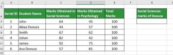
From the above table, we want to find the Social Sciences marks of Dsouza. However, we have not mentioned whether it is Alexa Dsouza or Ava Dsouza. As a result, we must add the value attributed to each Dsouza using the wildcard character Asterisk (*).
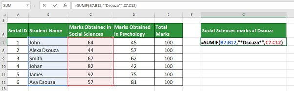
Step 2: Place the cursor in cell G7 and enter the formula,
=SUMIF(B7:B12,”*Dsouza*”,C7:C12)
Note: In Microsoft Excel, we use wildcard characters asterisk (*) mark and a question mark (?) more commonly.
Step 3: Press the Enter key to get the below result
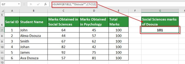
The SUMIF function returns the total marks for Dsouza as 101.
Explanation: We have written “*Dsouza*” instead of “Dsouza,” where the asterisk (*) searches for specific characters. Thus, it treats both Alexa Dsouza and Ava Dsouza as one and does the summation of Social Sciences marks for both students.
Sumif in Excel with Multiple Criteria
In the SUMIF function, we can add two criteria in a single range, i.e., we can use SUMIF for Multiple criteria. Let us understand this with some examples.
Using SUM with SUMIF function:
Example #1
Consider the same data as Example #1. Here we want to find the Total Sales value for France and Canada.
Step 1: Write Total Sales for France and Canada in cell A26
Step 2: Place the cursor in cell F26 and enter the formula,
=SUM(SUMIF(B7:B24,{“France”,”Canada”},F7:F24))
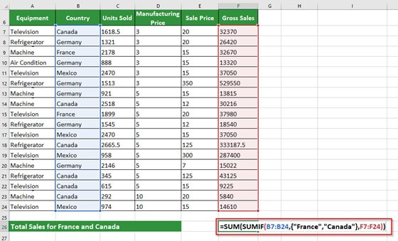
Explanation: Firstly, we put the SUM function before adding the function SUMIFS as we want to give two criteria(conditions) in the formula.
- The first parameter of SUMIF is criteria_range, i.e., B7:B24.
- We will enter the names of desired countries as the second parameter. Since we are giving multiple criteria, we must first enter curly brackets {} to include it.
- Inside the curly brackets {}, we must specify the desired country names in double quotes.
- The last part is sum_range, i.e., F7:F24.
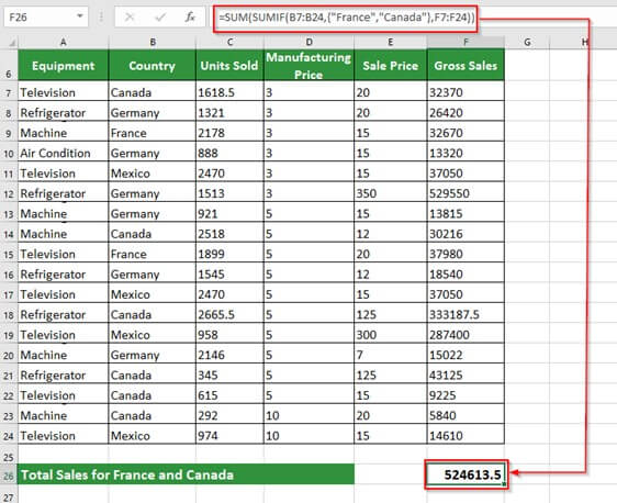
Firstly, SUMIF calculates the sales for France (70,650) and then calculates the sales for Canada (4,53,964). When SUMIF returns the total sales for both countries, the SUM function will add the two sales to give the output (70,650 + 4, 53, 964) as 524613.5.
SUMIF Multiple Criteria with OR Logic:
Example #2
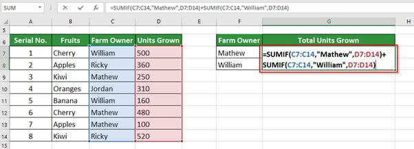
The table below displays a list of fruits, their farm owners, and the units grown per quarter. We want to know how many fruits the farm of Mathew and William has produced.
Step 1: Merge the cells G7 and G8
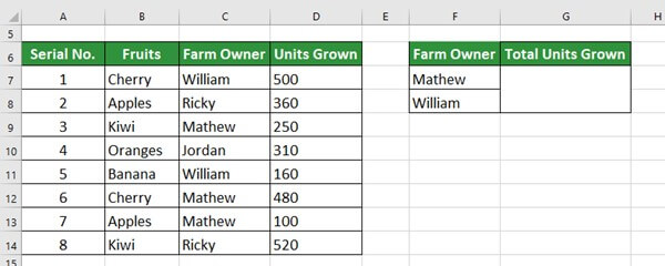
Step 2: Place the cursor in the merged cell and enter the formula,
=SUMIF(C7:C14,”Mathew”,D7:D14)+SUMIF(C7:C14,”William”,D7:D14)
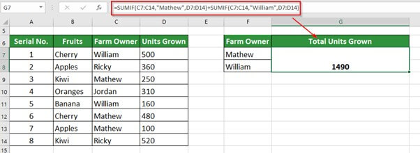
Step 3: Press the Enter key to get the below result
Sum with multiple AND criteria
Example #3
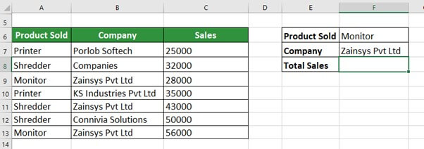
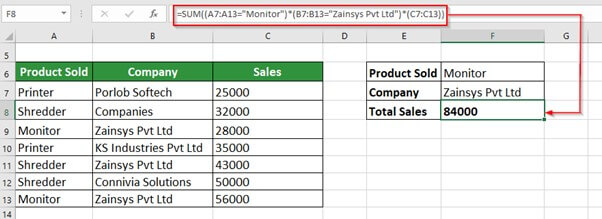
The table below shows office equipment sold to respective companies with the sales made in January 2023. We want to calculate the total sales of Monitor by Zainsys Pvt Ltd.
Step 1: Write Total Sales in cell E8
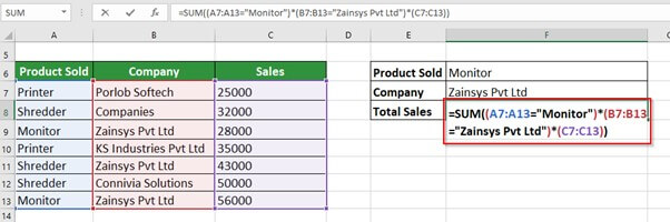
Step 2: Place the cursor in cell F8 and enter the formula,
=SUM((A7:A13=”Monitor”)*(B7:B13=”Zainsys Pvt Ltd”)*(C7:C13))
Step 3: Press the Enter key to get the result shown below
Difference between SUM vs. SUMIF in Excel
- The function SUM adds up multiple values, while the SUMIF function adds up multiple values which meet given criteria
- The syntax for the SUM function is
- The syntax for SUMIF is
Difference between VLOOKUP and SUMIF in Excel
- The VLOOKUP is a function in Excel that works as a search function.
- It can search for a particular value across a given range of columns.
- Hence, vlookup is not a math function like SUMIF in Excel
- The syntax for VLOOKUP is
=VLOOKUP(lookup_value, table_array, col_index_num, [range_lookup])
What is Nested SUMIF in Excel?
- A Nested SUMIF function sums up multiple values that meet multiple given criteria
- We can write Nested SUMIF as SUMIFS in Excel.
- A Nested SUMIF is also known as a Nested Loop.
- The syntax for Nested SUMIF or SUMIFS is
=SUMIFS(sum_range, criteria_range1, criteria1, [criteria_range2, criteria2],…)
Frequently Asked Questions (FAQs)
Q1) What does the SUMIF function of MS Excel do?
Answer: The SUMIF function in ms excel is used to add the values of a range corresponding to a particular value in a different range. The SUMIF is another function that checks the criteria before adding the values.
Q2) How to apply the SUMIF formula in Excel?
Answer: To apply the SUMIF formula in Excel, select a cell, type =SUMIF, and double-click the SUMIF option. Then we must write the first cell range that will work as the conditions and type a comma. Next, we must mention the criteria and then type a comma. Finally, we must add the cell range that we want to add.
Refer to the image below to understand the steps in a better way.
Q3) How to use the SUMIF function in excel with multiple sheets?
Answer: We can use the SUMIF function in Excel to perform calculations across multiple sheets using SUMIFS, SUMPRODUCT, and INDIRECT functions. The syntax for the same is-
SUMPRODUCT(SUMIFS(INDIRECT(“‘”&sheet_range”’!”&”sum_range),INDIRECT(“‘“&sheet_range&”’!”&”range”),data))
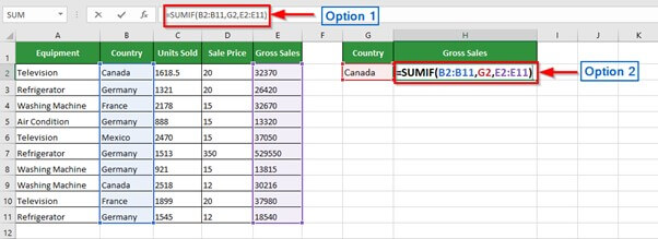
Q4) How to find SUMIF in Excel?
Answer: We can find SUMIF in Excel by simply writing =SUMIF in the formula bar or typing it directly in the cell where we want to store the value of the calculation.
The below image shows the two options where you can find the function SUMIF in Excel.
Q5) When do we use SUMIF in Excel?
Answer: We use SUMIF in Excel to add those values of a data range that meet certain criteria. We can use SUMIF to add values with multiple criteria by combining other functions such as SUMIFS and SUMPRODUCT.
SUMIF Function in Excel Video
Recommended Articles
The article has been a guide to SUMIF in Excel. Here, we discuss the SUMIF Formula and how to use SUMIF Function along with Excel examples and downloadable Excel templates. You may also look at these useful functions in Excel-