Excel Substring Function (Table of Contents)
Substring Function in Excel
Substring is how to extract some of the text from the cell in Excel. In Excel, we do not have any Substring function, but we can use LEN, Left, Right, Mid, Find function to slice the value there in a cell. For using Substring, we need to start the function with Left or Right and then select the cells from where we need to get the text, use the LEN function to get the length of characters we want to extract, then subtract the remaining characters using FIND function. By this, we will get Substring.
The LEFT, RIGHT, and MID functions are categorized under the TEXT function, which is inbuilt.
It helps us to:
- To get a string of any text.
- To find out a specifically required text of any string.
- To find out the position of any text in a string.
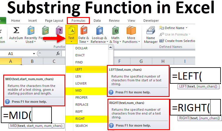
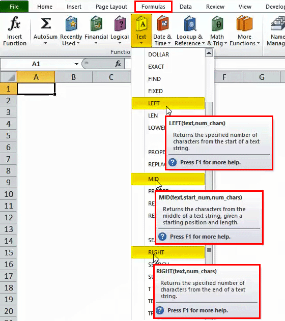
We can find these functions under the Formulas Tab.
Below is the screenshot for navigation purposes:
So, the above three are the most commonly used functions to find out the string for text.
How to Use Substring Function in Excel?
The substring function in Excel is very simple and easy to use. Let’s understand the working of the Substring function in Excel with some examples.
#1 – LEFT Function in Excel
LEFT Function helps the user to know the substring from the left of any text. It starts counting with the leftmost character.
The syntax or formula for the LEFT function in Microsoft Excel is:
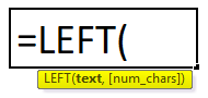
The LEFT function syntax or formula has the below-mentioned arguments:
- Text: This argument is compulsory as it represents the text from where we want to extract the characters or cell address.
- Num_chars: This one is an optional argument representing the number of characters from the text’s left side of the character we want to extract.
Extract a Substring in Excel Using the LEFT Function
Suppose we want the first two characters or substring from the given an example below screenshot:
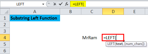
In cell C4, a text is given from which we want the first two characters. We have to type =LEFT and then use ( or press Tab in D4; look at the screenshot for reference:
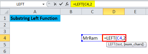
Now, we can see the argument required in the screenshot as well. We have to type or navigate the cell address to C4, and in place of num_chars, we need to put the number of characters we want; in this case, two characters are required, so we put 2.
Below is the screenshot for the above step:
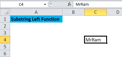
After putting an argument, we need to press ) or press Enter to get the result. Below is the screenshot after completing the formula.
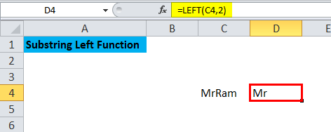
So, the result is Mr which is two characters of MrRam from the left. To extract the substring from the left, we can use the LEFT function in Excel.
Points to Remember while using LEFT Function in Excel
- The result or return value depends on the arguments inserted in the syntax.
- If the argument is less than (num_chars) 0, the result would be a #VALUE error.
- The output or return value can be string or text.
- An Excel LEFT function is used to extract the substring from the string, which calculates from the leftmost character.
#2 – RIGHT Function in Excel
The RIGHT function from Text also helps to get the substring from the rightmost of a text. If we do not put a number, it will show one character of the rightmost.
The syntax or formula for the RIGHT function in Microsoft Excel is:
The RIGHT function syntax or formula has the below-mentioned arguments:
- Text: The text string contains the characters where you want to extract them.
- num_chars: The number of characters from the RIGHT side of the text string you want to extract.
Extract a Substring in Excel Using RIGHT Function
Suppose we have to extract the last two characters of a word as shown in the below example:
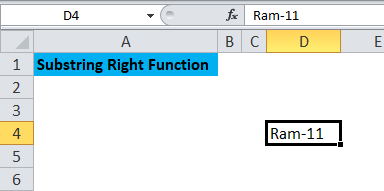
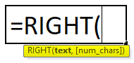
Suppose we have to find out the last two characters of the D4 cell, then type =RIGHT in E4. Below is the screenshot for reference:
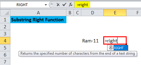
After that, we have to click on Tab or press (
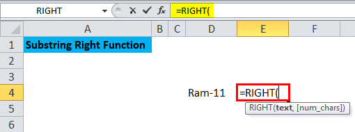
We can see that the required argument is populating in the above screenshot. Accordingly, on the place of text, put the cell address, which is D4, here, and we want two 2 characters from the right to put 2. Below is the screenshot for reference:
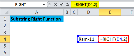
After putting all the arguments close, the formula by pressing ) or hitting Enter to know the result.
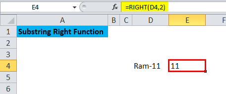
Hence, we can see in the above screenshot that 11 is populated after hitting Enter; the formula captures the last two characters from the right as entered in the argument. RIGHT Function helps to get the string from the right side of any character.
Points to Remember while using RIGHT Function in Excel
- The output depends on the syntax.
- The output will be a #VALUE error if the parameter exceeds (num_chars) 0.
- The result can be a string as well as text.
#3 – MID Function in Excel
It helps us extract a given number of characters from the middle of any text string.
The syntax or formula for the MID function in Microsoft Excel is:
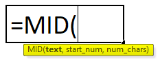
The MID function syntax or formula has the below-mentioned arguments:
- Text: The original text string or character from which we must extract the substring or characters.
- Start_num: It indicates the position of the first character where we want to begin.
- num_chars: The number of characters from the middle part of the text string.
Like the LEFT and RIGHT functions, we can use the MID function to get the text substring in Excel.
Extract a Substring in Excel Using the MID Function
Suppose, in the below example, we want to extract the three characters from the middle of the text, then we can use the MID Function.
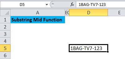
We will see how to use the MID Function to extract the string in the middle of cell E5, step by step.
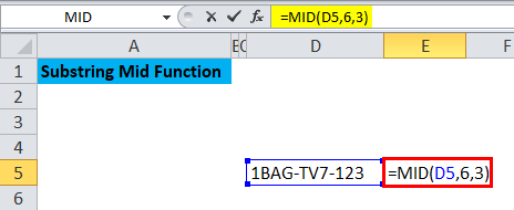
We have to type =MID and then press Tab or press ( like shown in the below screenshot.
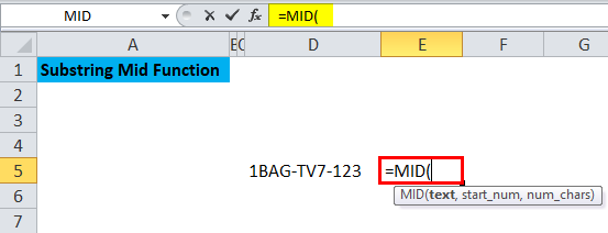
Now, we must enter the arguments shown in the above pic.
In place of text, we have to enter the cell address, which is D5 here, start_num is the argument that defines from where we want the string, so in this case, we want it from 6th from left, and the last argument is num_chars, which represents about the number of character we want, so here it is 3.
So, in the screenshot, we can see that argument is put down as per requirement. After putting an argument, close the formula with “)” or just hit Enter to get the results. Below is the screenshot for reference.
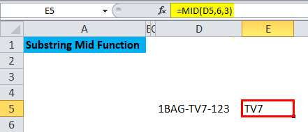
So, in the above screenshot, the TV7 results from the MID Function applied. TV7 is the three characters from the 6th position of the text as an example.
Things to Remember about Substring Function in Excel
- Simply use the substring function to obtain the phone number or code as needed.
- You can use the substring function to obtain the domain name of the email ID
- While using a substring in Excel, the text function needs to be conceptually clear to get the desired results.
- An argument should be put down in the formula as per the requirement.
Recommended Articles
This has been a guide to Substring Function in Excel. Here we discuss how to use Substrings functions in Excel – LEFT, RIGHT, and MID Functions along with practical examples and a downloadable Excel template. You can also go through our other suggested articles –
