Updated May 20, 2023

Introduction of NumPy fft
Python’s NumPy.fft() function computes the n-point DFT (Discrete Fourier Transform) of a single-dimensional signal. It employs the fast Fourier transform algorithm to calculate the frequency domain representation of the signal efficiently. This package provides the basic functions that are necessary for the manipulation of large arrays and makes cases that contain both alphanumeric and numeric data. To utilize the fast Fourier transform function, you can make use of the SciPy package, which is a subset of the larger NumPy library. SciPy provides additional scientific computing functionality and extends the capabilities of NumPy.
Syntax and Parameters
FFT() while writing codes in the Python programming language:
numpy * . * fft *. * fft * (* a1 *, * n1 * = * None *, * axis * = * -1 *, * norm * = * None *) *Parameters:
FFT() function written in the Python programming language:
Parameters:
- A1: array_like: Is used to represent the data that has been entered into the system by the programmer or entered by the user, which is the other process with the use of the function
- n1 int, optional: It is used to represent the actual length of the transformed after the array has been processed in the output. If the size of the array entered by the user is comparatively smaller than the output length, then the system provides the input array using 0’s. If a parameter is not specified in the syntax while writing the code, the default behavior is to use the size of the value entered along the fixed axis.
- Existing, optional: The parameter represents the axis of the array over which the fast frontier transformation is to be executed. Suppose the parameter is not specified in the syntax for the code.
- norm{None, “ortho”}, optional: This parameter is used to represent the normalization mode, specifically present in the systems that are using Python version 1.1.1.0 and above.
- optional: The parameter represents the axis of the array over which the fast frontier transformation is to be executed. If a parameter is not specified in the syntax of the code, the default behavior is to use the last axis of the input.
- Returns: This parameter represents the truncated input or the input with no padding. Python’s NumPy.fft() function computes the n-point DFT (Discrete Fourier Transform) of a single-dimensional signal.
How does the NumPy fft Work Systemically?
The FFT function, which uses the functionality of the SciPy package, works in a way that uses the basic data structures used in the numpy arrays to create a module required for scientific calculations and programming. This package helps utilize the functionalities that involve the functioning of linear algebra and calculus (differentiation and integration), the complexity of differential equations, and the dynamic versatility of the signaling processes.
Additionally, you also allow the user to check the in terms of its frequency and perform additional functions in the frequency domain.
Example of NumPy fft
An example displaying the use of NumPy.save() in Python:
Code:
# Python code example for usage of the function Fourier transform using the numpy.fft() method
import numpy as n1
import matplotlib.pyplot as plotter1
# Let the basal sampling frequency be 100;
Samp_Int1 = 100;
# Let the basal samplingInterval be 1
# The begin time for the time sampling of the process is taken as 0
Begin_Time1 = 0;
# Let the endtime period be 10 seconds
End_Time1 = 100;
# The final frequency being recorded for the signals
Signal_1Frequency     = 40;
Signal_2Frequency     = 70;
# Time points awarded are
time1 = n1.arange(begin_Time1, end_Time1, samp_Int1);
# Creation of2sinusoidal waves being done
amp1 = n1.sin(2*n1.pi*signal_1Frequency*time1)
amp2 = n1.sin(2*n1.pi*signal_2Frequency*time1)
# Creation of a sub plot being executed
figure1, axis1 = plotter1.subplots(4, 1)
plotter1.subplots_adjust(hspace=1)
# The time domain has a representation for sinusoidal wave 1
axis[0].set_title('Sine wave with a frequency of 4 Hz')
axis[0].plot(time, amplitude1)
axis[0].set_xlabel('Time')
axis[0].set_ylabel('Amplitude')
# Time domain representation for sine wave 2
axis[1].set_title('Sine wave with a frequency of 7 Hz')
axis[1].plot(time, amplitude2)
axis[1].set_xlabel('Time')
axis[1].set_ylabel('Amplitude')
# Add the sine waves
amplitude = amplitude1 + amplitude2
# Time domain representation of the resultant sine wave
axis[2].set_title('Sine wave with multiple frequencies')
axis[2].plot(time, amplitude)
axis[2].set_xlabel('Time')
axis[2].set_ylabel('Amplitude')
# Frequency domain representation
fourierTransform = np.fft.fft(amplitude)/len(amplitude)           # Normalize amplitude
fourierTransform = fourierTransform[range(int(len(amplitude)/2))] # Exclude sampling frequency
tpCount     = len(amplitude)
values      = n1.arange(int(tpCount/2))
time_Period1  = tpCount/samp_Fre1
frequencies1 = values/time_Period1
# Frequency domain representation
Axis1[3].set_title('Fourier transform depicting the frequency components')
Axis1[3].plot1(frequencies1, abs(fourierTransform))
Axis1[3].set_xlabel('Frequency')
Axis1[3].set_ylabel('Amplitude')
plotter1.show()
Output:
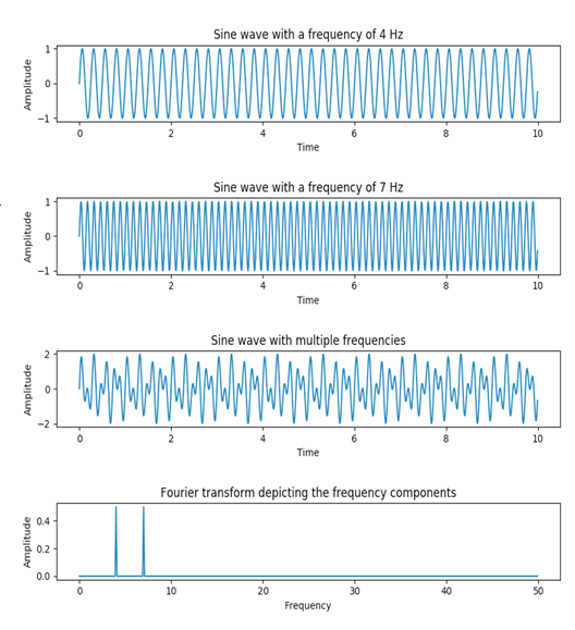
The fft() function converted the sinusoidal wave, which had frequencies of 4 Hz and 7 Hz, into a single wave that combines multiple frequencies. The transformed wave represents the frequency component using the function, which measures the wave’s vital parameters in terms of frequency, including frequency itself and amplitude.
Conclusion
The NumPy.fft() has a multifaceted functionality. The occasion range varies in its usage, including processing voice signals and deviant signal processing procedures. The bike is one of the most utilized concepts concerning the Digital Signal Processing domain, especially when used in the sinusoidal domain. The versatile approach of the function allows for the transformation of both periodic and non-periodic signals from the time domain to the frequency domain.
Recommended Articles
We hope that this EDUCBA information on “NumPy fft” was beneficial to you. You can view EDUCBA’s recommended articles for more information.