Updated August 10, 2023
MIRR in Excel (Table of Contents)
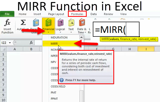
MIRR in Excel
MIRR function under the financial category is a unique statistical function that provides the interest rate on invested amount and finds a series of net income against the invested amount. For using MIRR, we must have a series of investments, finance rate, and reinvest rate, and the argument should contain at least one positive and one negative value.
MIRR Formula in Excel
The Formula for the MIRR Function in Excel is as follows:
The MIRR function syntax or formula has the below-mentioned arguments:
- Values: It is a cell reference or array which refers to the schedule of cash flows, including the initial investment with a negative sign at the start of the stream
Note: The array must contain at least one negative value (initial payment) and one positive value (returns). Here negative values are considered payments, whereas Positive values are treated as income.
- Finance_rate: It’s the cost of borrowing or interest rate paid on the money used in the cash flows (negative cash flow)
Note: It can also be entered as a decimal value, i.e. 0.07 for 7%
- Reinvest_rate: It’s an interest rate that you receive on the reinvested cash flow amount (Positive cash flow)
Note: It can also be entered as a decimal value, i.e. 0.07 for 7%
MIRR FUNCTION helps separate negative & positive cash flows & discounting them at the appropriate rate.
How to Use MIRR Function in Excel
MIRR Function in Excel is very simple and easy to use. Let us understand the working of MIRR in Excel with Some Examples.
Example #1
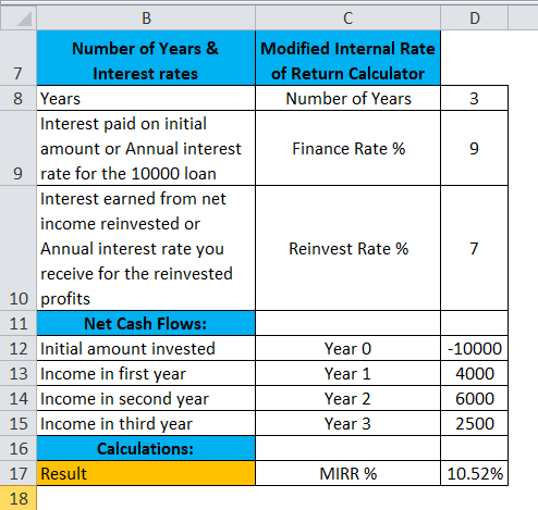
In the below-mentioned example, the Table contains the below-mentioned details.
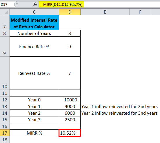
Initial investment: 10000, Finance rate for MIRR is 9% & Reinvestment rate for MIRR is 7%
Positive cash flow: Year 1: 4000
Year 2: 6000
Year 3: 2500
Using the MIRR Function, I need to determine the investment’s Modified Internal Rate of Return (MIRR) after three years.
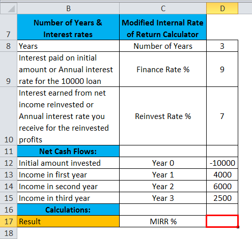
Let’s apply the MIRR function in cell “D17”.
Select the cell “D17” where the MIRR function needs to be applied; click the insert function button (fx) under the formula toolbar, and a dialog box will appear, type the keyword “MIRR” in the search for a function box, MIRR function will appear in select a function box.
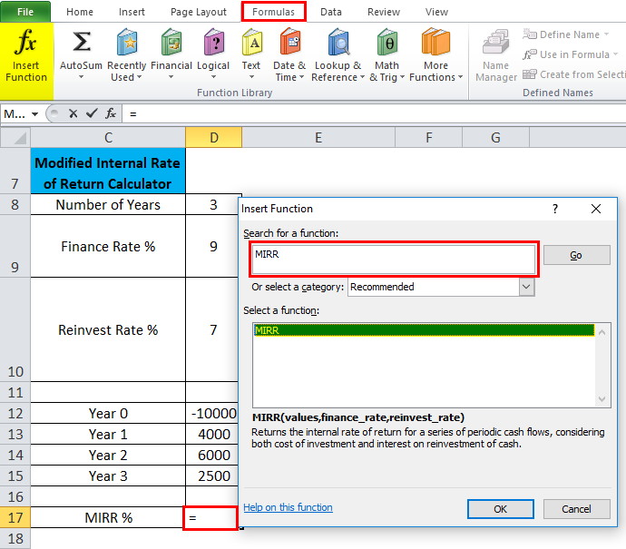
Double click on the MIRR function, and A dialog box appears where arguments for the max function need to be filled or entered, i.e. =MIRR(values, finance_rate, reinvest_rate
values argument: It is a cell reference or array which refers to the schedule of cash flows including the initial investment with a negative sign at the start of the stream. To select an array or cell reference, click inside cell D12 to see the cell selected, then Select the cells till D15. So that column range will get selected, i.e. D12:D15
finance_rate: It is the Interest paid on an initial amount or Annual interest rate for the 10000 loans, i.e. 9% or 0.09
reinvest_rate: Interest earned from net income reinvested or the Annual interest rate you receive for the reinvested profits, i.e. 7% or 0.07
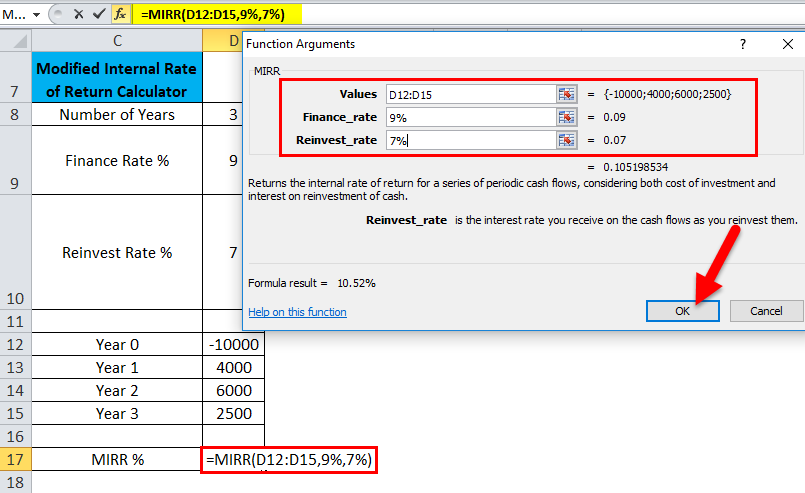
Click ok after entering the three arguments. =MIRR(D12:D15,9%,7%), i.e. returns the investment’s Modified Internal Rate of Return (MIRR) after three years. i.e. 10.52% in the cell D17
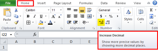
Note: Initially, it will return the value 11%, But to get a more precise value, We have to click on increase decimal place by 2 points. So that it will give an exact investment’s returns, i.e. 10.52%
Example #2
In the below-mentioned table, Suppose I want to choose one project from two given projects with the same initial investment of 100000.
Here I need to compare the Five-year modified internal rate of returns based on a 9% finance rate & reinvest_rate of 7% percent for both project with an initial investment of 100000.
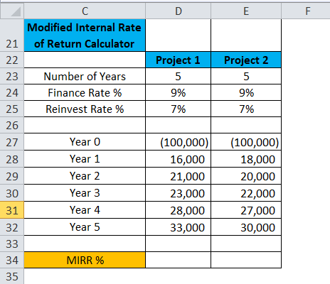
Let’s apply the MIRR function in cell “D34” for Project 1 & “E34” for Project 2.

Select the cell “D34” where the MIRR function needs to be applied; click the insert function button (fx) under the formula toolbar, and a dialog box will appear, type the keyword “MIRR” in the search for a function box, MIRR function will appear in select a function box.
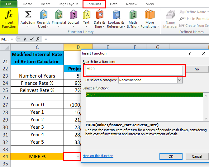
The above step is simultaneously applied in cell “E34.”
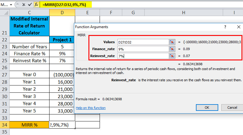
Double click on the MIRR function; a dialog box appears where arguments for the max function need to be filled or entered =MIRR(values, finance_rate, reinvest_rate) for project 1.
values argument: It is a cell reference or array which refers to the schedule of cash flows, including the initial investment with a negative sign at the start of the stream. To select an array or cell reference, click inside cell D27 to see the cell selected, then Select the cells till D32. So that column range will get selected, i.e. D27:D32
finance_rate: It is the Interest paid on an initial amount or Annual interest rate for the 10000 loans, i.e. 9% or 0.09
reinvest_rate: Interest earned from net income reinvested or the Annual interest rate you receive for the reinvested profits, i.e. 7% or 0.07
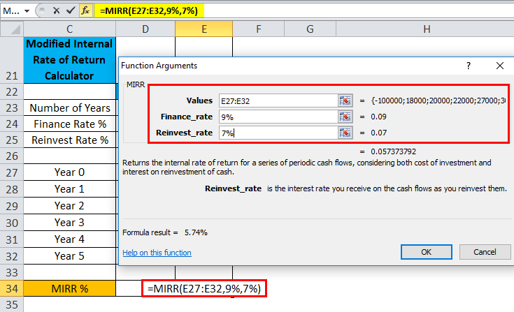
A similar procedure is followed for project 2 (Ref: Below mentioned screenshot)
Note: To get a more precise value, We have to click on increase decimal place by 2 points in cell D34 & E34 for both projects 1 & 2 So that it will give exact investment returns.

For project 1
=MIRR(D27:D32,9%,7%), i.e. returns the investment’s Modified Internal Rate of Return (MIRR) after three years. i.e. 6.34% in the cell D34
For project 2
=MIRR(E27:E32,9%,7%), i.e. returns the investment’s Modified Internal Rate of Return (MIRR) after three years. i.e. 5.74% in the cell E34
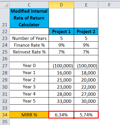
Inference: Based on the MIRR calculation, Project 1 is preferable; it has given better returns compared to Project 2
Things to Remember
- Values must contain at least one negative value & one positive value to calculate the modified internal rate of return. Otherwise, MIRR returns the #DIV/0! error
- If an array or reference argument contains empty cells, text or logical values, those values are ignored
- #VALUE! error occurs if any of the supplied arguments is not a numeric value or non-numeric
- Initial investment needs to be in a negative value; otherwise, the MIRR Function will return an error value (#DIV/0! Error)
- MIRR Function considers both the cost of the investment (finance_rate) and the interest rate received on cash reinvestment (reinvest_rate).
- The main difference between MIRR & IRR is that MIRR considers the interest received on the reinvestment of cash, whereas the IRR does not.
Recommended Articles
This has been a guide to MIRR in Excel. Here we discuss the MIRR Formula in Excel and how to use MIRR Function in Excel, along with Excel examples and downloadable Excel templates. You may also look at these useful functions in Excel –
