Updated August 16, 2023

Highlight Rows in Excel (Table of Contents)
Highlight Every Other Rows in Excel
Highlighting every other row in Excel is done using Conditional Formatting. This improves a user’s readability and helps distinguish the different rows from other data values. Select a new rule from the Conditional Formatting list, which is under the Home menu tab, and there we can use the MOD function along with ROW to reach every second row. And then, choose the color by which we want to highlight every other row in which we get the applied rule.
How to Highlight Every Other Row in Excel?
There are various methods of highlighting or shading every other row of your data in Excel.
Method 1 – Using Excel Table
This is the easiest and quickest way to highlight every other row in Excel. In this method, the default ‘Excel table’ option is used.
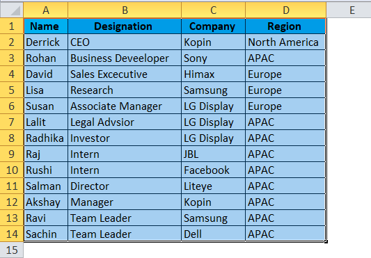
Consider the below example, where any random data is entered in the Excel sheet.

The steps to highlight every other row in Excel by using an Excel table are as follows:
Step 1: Select the entire data entered in the Excel sheet.
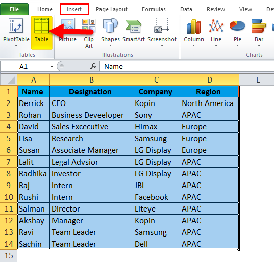
Step 2: From the ‘Insert’ tab, select the option ‘Table,’ or else you can also press ‘Ctrl +T,’ which is a shortcut to create a table.
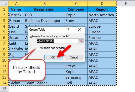
Step 3: You will get the ‘Create Table’ dialog after selecting or creating the table option. In that dialog box, clicks on ‘OK.’
This will create a table like this.

The figure above demonstrates the highlighting of every other row.
If you want your data to look or appear in a different style or format, select the ‘Table Styles‘ option from the ‘Design’ tab, as shown below.
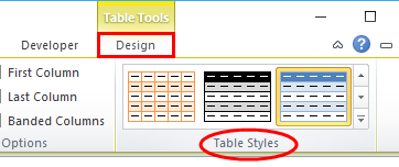
The below figure shows how modification could be done to your table by clicking the design tab, selecting the ‘Table Styles’ option, and selecting your preferred style. (Design->Table Styles)

Method 2 – Using Conditional Formatting
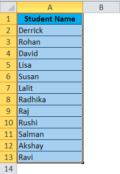
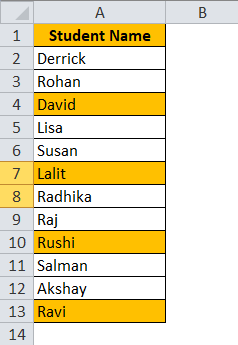
This method is useful when highlighting every Nth row in the spreadsheet. Consider the below example as shown in the figure.

In this example, a teacher needs to highlight every 3rd student and group them in one group. The steps to highlight every other row in Excel using conditional formatting are as follows:
Step 1: Select the data which needs to be highlighted.
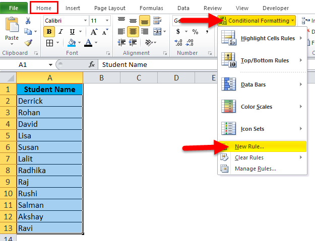
Step 2: Click on the ‘Home Tab’ and then the ‘Conditional Formatting’ icon. After clicking on conditional formatting, select the ‘New Rule’ option from the drop-down.
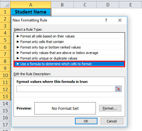
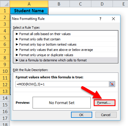
Step 3: After selecting the new rule, a dialog box will appear, from which you need to select ‘Use a formula to determine which cells to format.’
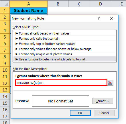
Step 4: Enter the formula in the empty box under the ‘Edit the Rule Description’ section. Formula is ‘=MOD(ROW(),3)=1’.
Understanding the Formula
The MOD formula returns the remainder when the ROW number is divided by 3. The formula evaluates each cell and checks if it meets the criteria. So, for example, it will check cell A3. Where the ROW number is 3, the ROW function will return 3, so the MOD function would calculate =MOD(3,3) which returns 0. However, this hasn’t met our designed or specified criteria. Hence, it moves to the next ROW.
The cell is A4, where the ROW number is 4, and the ROW function will return 4. So, the MOD function will calculate =MOD(4,3), and the function returns 1. This meets our specified criteria, and therefore, it highlights the entire ROW.
You can customize this formula based on your specific requirements. For example, consider the below modifications:
- The formula for highlighting every 2nd ROW starting from the 1st ROW would be ‘=MOD(ROW(),2)=0’.
- To highlight every 2nd or 3rd COLUMN, the formula would be ‘MOD(COLUMN(),2)=0’ and ‘MOD(COLUMN(),3)=0’ respectively.
Step 5: After that, click on the ‘Format’ button.
Step 6: After that, another dialog box will appear. From that, click the ‘Fill’ tab and select any color you like.
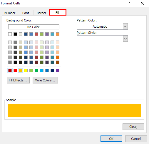
Step 7: Click OK. This will highlight every 3rd row of our data in Excel.
Advantages
In the case of conditional formatting, if you add new rows within range, the highlighting or shading of the alternate ROW would be done automatically.
Disadvantages
For a new user, it becomes difficult to understand the conditional formatting by using the formula for it.
Things to Remember about Highlight Every Other Row in Excel
- If you use the Excel table method or standard formatting option and need to enter a new ROW within range, the shading for alternate ROW will not automatically be done. It would be best if you did it manually.
- The MOD function can also be used for ROW and COLUMN. It would be best if you modified the formula accordingly.
- The color of the ROWs cannot be changed if conditional formatting is done. You need to follow the steps from first again.
- If a user needs to highlight both even and odd groups of ROWs, then the user needs to create two conditional formattings.
- Use light colors for highlighting if the data needs to be printed.
- In Excel 2003 and earlier versions, you can perform conditional formatting by clicking on the ‘Format’ menu and then selecting ‘Conditional Formatting.’
Recommended Articles
This has been a guide to Highlight Every Other Rows in Excel. Here we discuss how to highlight every other row in Excel using an Excel table, conditional formatting, practical examples, and a downloadable Excel template. You can also go through our other suggested articles –
