Updated August 21, 2023
Header Row in Excel
In this article, we will learn about Header Row in Excel. Microsoft Excel sheet can hold a million rows with a numeric or text dataset in it. In Excel or Word, the row header is the gray column on the left side (column 1) with numbers to identify each row, while the column header is the gray row with letters (A, B, C, etc.) to identify each column in the worksheet.
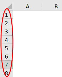
Row header labels will help you to identify & compare the information of the content when you are working with a huge number of data sets, when it is difficult to accommodate the data in a single window or page & to compare information in your worksheet of excel.
Usually, a combination of column letters and row numbers helps create cell references. The row header in Excel is crucial for cell identification.
Definition
Header rows are the label rows containing information that helps you identify the content of a particular column in a worksheet.
If the dataset table spans several pages in an Excel sheet print layout or towards the right if you scroll on & on, the header row will remain constant & stagnant, which usually repeats itself at the beginning of each new page.
How to Turn the Header Row on or off in Excel?
Row headers in Excel remain visible even when scrolling the column data set or values to the right in the worksheet.
Sometimes, the row header in Excel will not be displayed on a particular worksheet. It will be turned off in several cases. The main reason for turning them off is –
- Better or improved appearance of the worksheet in Excel or
- To obtain or gain the extra screen space on worksheets containing many tabular datasets.
- To take a screenshot or capture.
- When you take a printout of a tabular dataset, the row header or heading makes things complicated or confusing with the printed data set because of interference of the row & column header; When taking a printout in Excel, the row header should always be turned off for each individual worksheet.
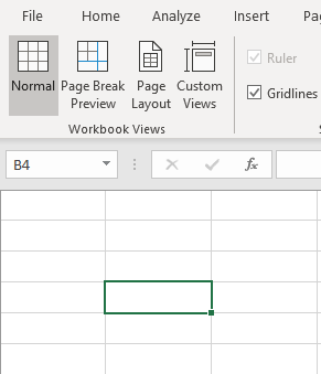
Now, let’s check out how to turn off Excel’s row headers or headings.
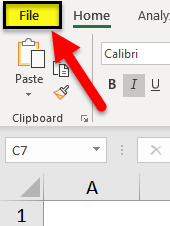
- Select or Click on the File option in the home toolbar of the menu to open the drop-down list.
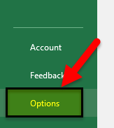
- Click on Options in the list present on the left-hand side to open the Excel Options dialog box.
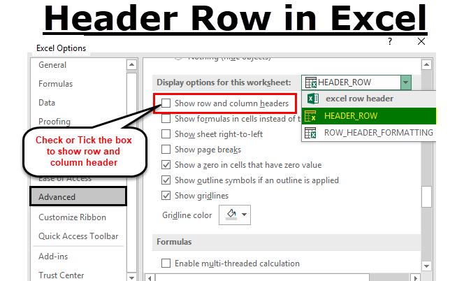
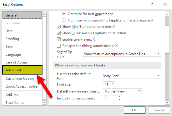
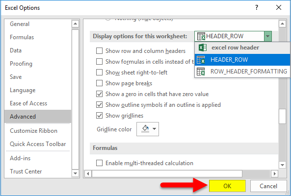
- Now, the Excel Options dialog box appears; in the left-hand panel of the Excel options dialog box, select the Advanced option.
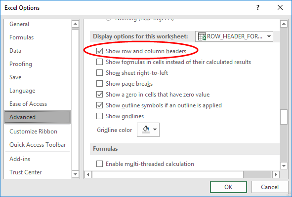
- Now, if you move the cursor down after the advanced option, you can observe Display options for this worksheet section located near the bottom of the right-hand pane of the dialog box; by default, it shows the row and column headers option always checked or ticked in.
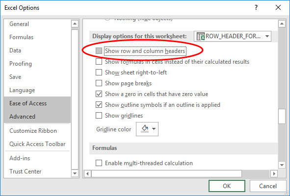
- If you want to turn off the row headers or headings in Excel, click on or uncheck the selection box of a checkbox in the Show row and column headers option.
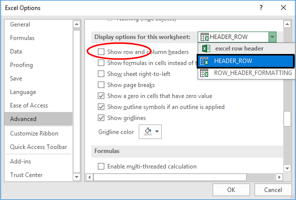
- Simultaneously, you can turn off the row and column headings for additional worksheets in the open workbook or the current workbook of Excel. It can be done by selecting the name of another worksheet under the drop-down box next to the Display options.
- Once you have unchecked the box, Click OK to close the Excel options dialog box, and you can return to the worksheet.
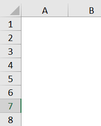
- Now, the above procedure disables the visibility of a row or column header.
Header Row Formatting Options in Excel
When you try to open a new Excel file, the row header or heading is displayed by default in a normal style or theme font similar to the workbook’s default format. This same normal style font also applies to all the worksheets in the workbook.
The default heading font is Calibri & the font size is 11. It can be changed based on your choice as per your requirement; whatever font style & size you apply will reflect in all the worksheets in a workbook of Excel.
You have the option to format font & its size settings, with various options in format settings.
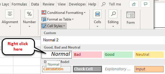
- In the Home tab of the Ribbon menu. Under the Styles group, select or click on Cell Styles to open the Cell Styles drop-down palette.
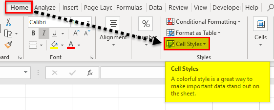
- In the dropdown, under Good, bad & Neutral, Right-click or select the box in the palette entitled Normal, also called a Normal style.
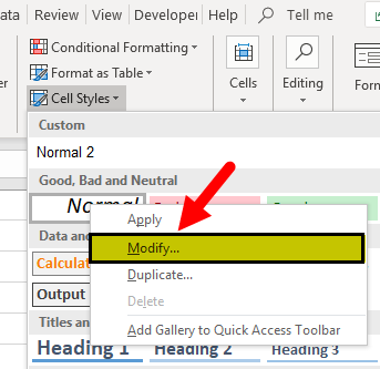
- Click on Modify option under normal.
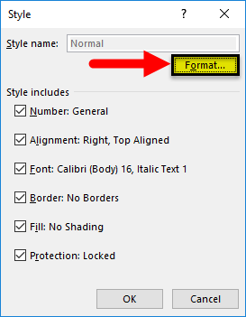
- A style dialog box appears; click on the Format in that window.
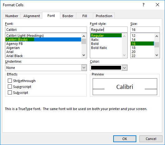
- Now, the Format Cells dialog box appears. In that, you can change the font size and appearance, i.e. Font style or size.
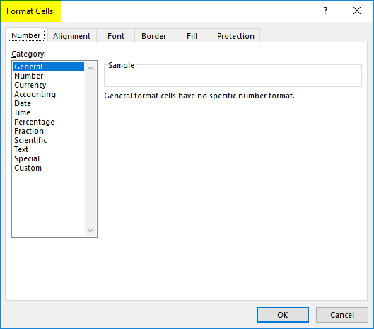
- I changed the font style & size, i.e. Calibri & font style, to Regular, and I increased the font size to 16 from 11.
Once the desired changes are made, click OK twice, i.e. in the format cells dialog box & style dialog box, based on your preference.
Note: Once you make changes in the font settings, you have to click on the save option in the workbook; otherwise, it will revert back to the default normal style or theme font (i.e.default heading font is Calibri & font size is 11).
Things to Remember
- Using row headers with row numbers in Excel can help with navigation and organization.
- The benefit of a header is that we can print it on all pages in Excel or Word.; it is very significant & will be helpful for spreadsheets that span multiple pages.
Recommended Articles
This has been a guide to Header Row in Excel. Here we discuss how to turn the row header on or off and row header formatting options in Excel. You can also go through our other suggested articles –
