Updated August 19, 2023
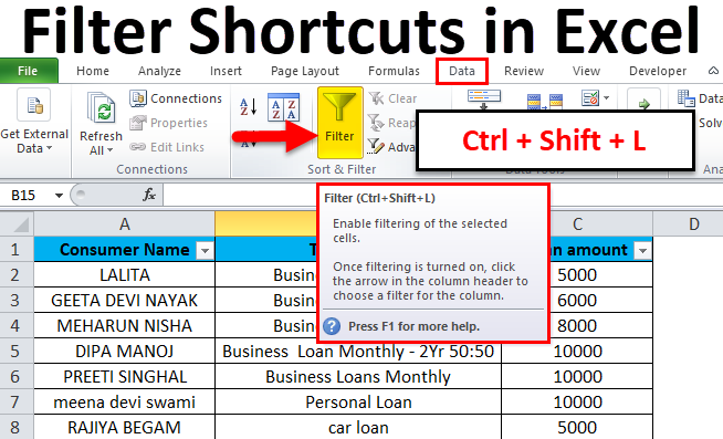
Filter Shortcuts in Excel
In this article, we will learn about Filter Shortcuts in Excel. there are different ways to access and apply filters in Excel. In the first way, we can select the headers first, then from the Data menu tab, select Filter Option under the Sort & Filter section. In a second way, we can apply the filter by pressing shortcut keys Alt + D + F + F simultaneously, and another way is by pressing shortcut keys Shift + Ctrl + L together to apply a filter in one go. Once the filter is applied, we can use other shortcut keys, such as the Alt + Down key, to get into the applied filter and select an option by pressing a shortcut key or navigation keys.
How to Use Filter Shortcuts in Excel?
Filter Shortcut in Excel is very simple and easy to use. Let’s understand the working of filter shortcuts in Excel with some examples.
#1 – Toggle Autofilter in the ribbon
Example #1
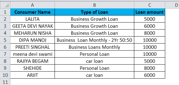
Here is a sample data on which we have to apply a filter.
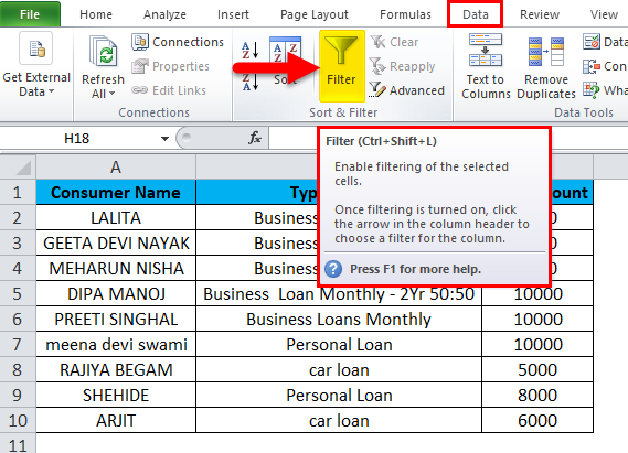
- We have to first click on the Data tab and then click on Filter, as shown below.
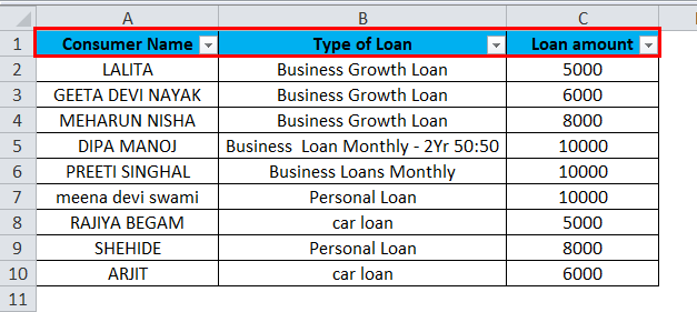
- Once we click the Filter tab on the ribbon, we will see that filter is applied to the data, that is, on all the columns.
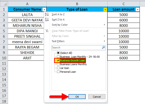
- Now, if we want to see the name of consumers who have taken a Business Growth Loan, we can select Business Growth Loan in the filter drop-down and then click on OK as shown below:
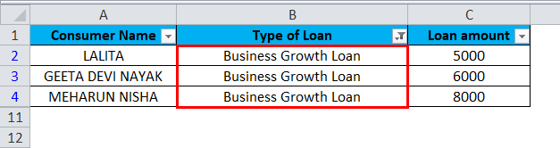
- You will see the name of the consumers who have taken Business Growth Loan.
- To disable Filter, you need to again click on the Filter in Ribbon in MS Excel.
Example #2
- Now, if we want to see how many consumers have taken a loan of 10000, we can apply the filter as shown below:
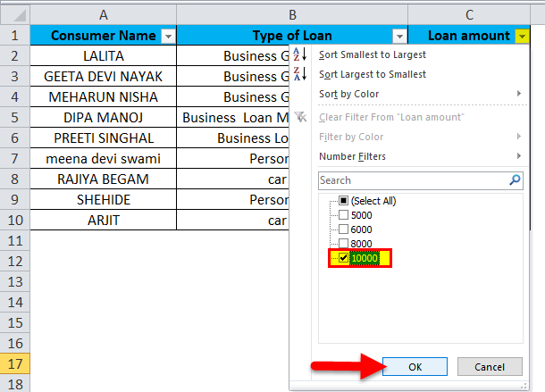
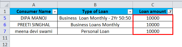
- On clicking Ok. You will then be able to filter the data as per your requirement.
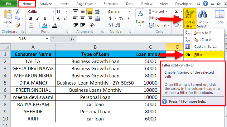
#2 – Applying filter using the “Sort and Filter” option on the Home tab in the Editing Group
It can be found on the right side of the Ribbon in MS Excel.
Using the above data, here is how we can apply the filter:
- To apply a filter, click on Sort & Filter, then click on the Filter option, the fourth option in the dropdown.
Example #3
- To filter the consumers who have taken a car loan.
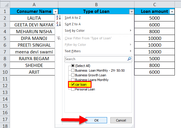
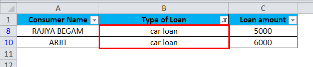
- On clicking Ok. You will see the consumers who have taken a car loan.
Example #4
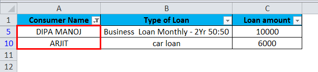
Now, if we need to filter some particular consumers, like their loan amount and their loan type, suppose we want to know the above details for Arjit and Dipa; we will apply the filter as below:
- Select Arjit and Dipa Manoj in the filter dropdown and click Ok.
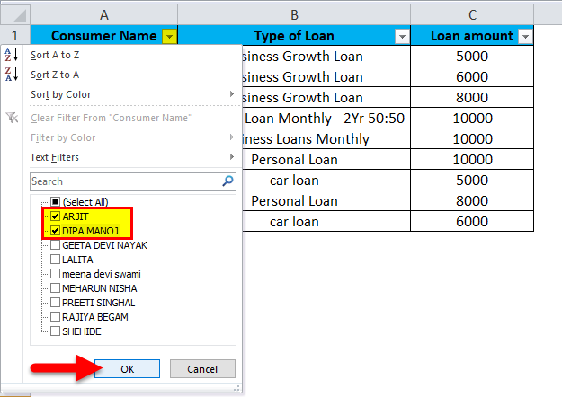
- We will then be able to see the relevant details.
- You can disable the filter on the data by clicking on the Sort and Filter option.
#3 – Filter the Excel data by Shortcut Key
We can rapidly press a shortcut key to apply the filter to our data. Together, we have to press Ctrl+shift+L.
Example #5
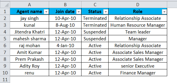
Here is a sample data on which we have applied the filter using the shortcut key.
- Select the data and then press the shortcut key to apply the filter, i.e., Ctrl+shift+L.
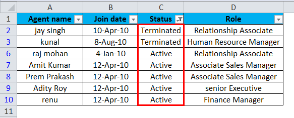
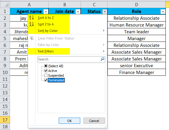
- If we want to filter the status of the Agents, like Active and Terminated, from the complete data, we will proceed as below:
- Press OK, and we will see the Active and Terminated agents.
While applying filters on the selected criteria, we see other options as well as shown below:
On top of the filter drop-down, we see an option Sort A to Z; then we have Sort Z to A, Sort by color, and Text filters.
Let’s look into these options. If we click on Sort A to Z, this is how we see the data:
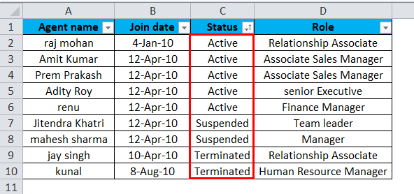
The data is filtered and got sorted in order of A to Z. Likewise if we click Sort Z to A, we will see the data as below:
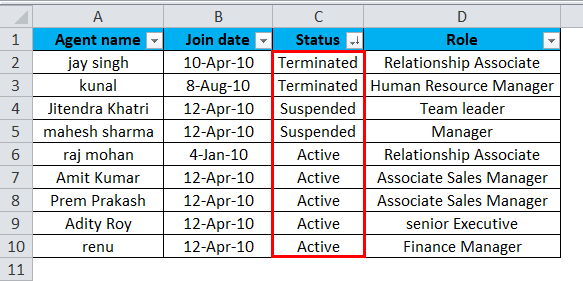
The data is filtered and sorted in order of Z to A.
By clicking Sort by color, the data will be filtered as per our criteria and sorted as per the color of that cell; if you select a cell colored red, that will be on the top.
And, if we click Text Filter:
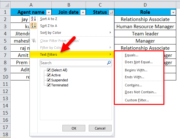
We get an option for an advanced filter for text, such as:
- Filter cells that Begin with or End with a specific text or character.
- Filter cells that Contain or Do not Contain a particular text or symbol.
- Filter cells that are either Equal to or Do not equal to a specific text or characters.
When we click on Does not equal to option and write Suspended in the dialogue box as shown below:
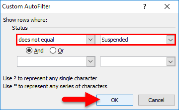
After we click “Ok”, we will see the data filtered as:
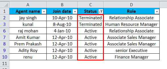
The data shows only Active and terminated status and not suspended.
Once you have applied the filter, you can disable it from that column as shown:
- Once we click Clear Filter from “Status”, the filter will be cleared from the Status column of the data.
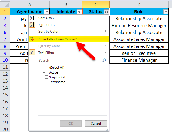
To remove a filter from the whole data, again press Ctrl+Shift+L.
Once you have filtered the data, copy it to any other worksheet or workbook. You can select the filtered data or filtered cells by pressing Ctrl + A. Then Press Ctrl+C to copy the filtered data, go to another worksheet/workbook, and paste the filtered data by pressing Ctrl+V.
Things to Remember About Filter Shortcuts in Excel
- Some Excel filters can be used one at a time. For Example, you can filter a column by either value or color at a time and not with both options simultaneously.
- For better results, avoid using different value types in a column. As for one column, one filter type is available. If a column contains different types of values, the filter will be applied for the high-frequency data. For example, if the data is in number in a column but is formatted as text, then the text filter will be applied, not the number filter.
- Once you have filtered a column and pasted the data, remove a filter from that column because the next filter in a different column will not consider that filter, and hence the filtered data will be correct.
Recommended Articles
This has been a guide to Filter Shortcuts in Excel. Here we discuss how to use Excel filter shortcuts, practical examples, and a downloadable Excel template. You can also go through our other suggested articles –
