Updated May 12, 2023
![]()
Introduction to Icon Sets in Excel
Icon Sets in Excel are the sets of the different types of Icons, Shapes, Indicators, and Directions, which are used for visualizing the selected values by giving them different meanings to them. Icon Sets can be accessed by the Home menu ribbon’s conditional formatting drop-down list. There we will have different categories, and all the icons on the list have some purpose and use. We can use directions for ups and downs in data; for any indications, use Shapes and Indicators and rate anything, prefer Ratings.
How to Use Icon Sets in Excel?
Using Icon Sets in Excel is easy, and we can find the icon sets in the Home menu under the Conditional Formatting styles group, shown by examples.
Example #1
Applying Indicator Icon Sets Using Conditional Formatting
In Microsoft Excel, there are icon sets with different shapes, and Icon sets in Excel are a unique kind of conditional formatting. Here in this example, we will see how to use indicator icon sets in Excel using conditional formatting.
Consider the below example, which shows the purchase date of Nov-16 month.
![]()
In this example, we will apply indicator icon sets in Excel using conditional formatting, where our conditional formatting formula is as follows.
- Green Colour Icon: If the value exceeds or equals 811.
- Yellow Colour Icon: If the value is less than 811 and greater than equal to 250 percent.
- Red Colour Icon: If the value is less than 250 percent.
In this example, we will see how to display these icon sets in Excel by following the process below.
- First, create a new column for displaying icon sets, as shown below. Then next, apply the = (equal) sign in I2 and select the G2 cell to get the value in the I2 cell for applying conditional formatting.
![]()
- Drag down the formula to all cells so that we will get the values shown in the screenshot below.
![]()
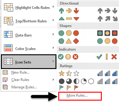
- Next, select the full column name Icon Set, click on Conditional Formatting, and select Icon Sets to get the option to choose the icon shapes as shown below.
![]()
- Once we click on the icon sets in Excel, we will get various icons like Directions, Shapes, Indicators, and Ratings.
- In this example, we will choose the flag icon set indicators to display the output.
- In the icon sets at the bottom, we can find “More rules”, where we can apply conditional formatting.
- On top of that, we can see various format rules. Please select the first format rule Format all cells based on their values.
- We can see the format, Icon, and Icon to be displayed in the above dialogue box. Now apply the conditional formatting as below so that we will get the icon sets to be displayed.
- Green Colour Icon: if the value exceeds or equals 811.
- Yellow Colour Icon: if the value is less than 811 and greater than equal to 250 percent.
- Red Colour Icon: if the value is less than 250 percent.
- Change the icon style to Flag. Apply the values and choose the Type as a Number because, by default, excel will take the values as a percent. We have chosen the type as a number because the format rule is based on values, not the percentage shown in the screenshot below.
![]()
- Click OK, and we will get the below output as follows.
![]()
- The above screenshot shows that icon set Flag indicators are displayed based on the condition we have applied.
- As we notice that icon sets are displayed along with the values. In order to display only the icon, we need to select the Show Icon Only check box option.
- Go to conditional formatting and choose icon sets to get the dialog box below.
![]()
- In the above screenshot, we can see that the checkbox is enabled for “Show Icon Only” to remove all the values and display the output with only the selected icons set, shown as the output result below.
In the below result, we can see the flag icon in column I, where we have applied a condition to display as Green Flag: If the value is greater than or equal to 811 and Yellow Flag: if the value is less than 811 and greater than or equal to 250 and Red Flag: if the value is less than 250.
![]()
Example #2
Applying Direction Icon Sets Using Conditional Formatting
In this example for Icon sets in Excel, we will apply the Direction Icon Set in Excel by using the same condition formatting.
Consider the below example, which shows sales data value for May-18. In this example, we will check which product has sold out with the highest value using the icon set conditional formatting by following the steps below.
![]()
In this example, we will apply Direction icon sets (High & Low) using conditional formatting, where our conditional formatting formula is as follows.
- Green Colour Icon: if the value is greater than or equal to 45000.
- Yellow Colour Icon: if the value is less than 45000 and greater than or equal to 43000.
- Red Colour Icon: if the value is less than 0.
In this example, we will see how to display these icon sets by following the steps below.
- First, create a new column for displaying icon sets, as shown below.
- Then apply the = (equal) sign in the I2 column and select the G2 cell to get the value in the I2 cell for applying conditional formatting.
![]()
- Drag down the formula to all cells so that we will get the values shown in the screenshot below.
![]()
- Next, select the full column of Icon Sets. Click on Conditional Formatting and select icon sets so that we can choose the icon shapes as shown below.
![]()
- Once we click on the icon sets, we will get various icons like Directions, Shapes, Indicators, and Ratings.
- In this example, we will choose the Direction icon set indicators to display the output.
- In the icon sets at the bottom, we can find more rules to apply conditional formatting here.
- Click on More Rules to get the conditional formatting dialog box as follows.
- On top of that, we can see various format rules. Then select the first format rule Format all cells based on their values.
- We can see the format style, Icon style, and icon to be displayed in the above dialogue box. Now apply the conditional formatting as below so that we will get the icon sets to be displayed.
- Green Colour Icon: if the value is greater than or equal to 45000.
- Yellow Colour Icon: if the value is less than 45000 and greater than or equal to 43000.
- Red Colour Icon: if the value is less than 0.
- Change the icon style to the Direction icon. Apply the values and choose the type as a Number because, by default excel will take the values as the percent. We have chosen the type as a number because the format rule is based on values, not the percentage shown in the screenshot below.
![]()
- Click OK, and we will get the below output as follows.
![]() The above screenshot shows that icon set Direction indicators are displayed based on the condition we have applied.
The above screenshot shows that icon set Direction indicators are displayed based on the condition we have applied.
- As we notice that icon sets are displayed along with the values. To display only the icon, we must select the Show Icon Only checkbox option.
- Go to conditional formatting and choose icon sets to get the dialog box below.
![]()
- In the above screenshot, we can see that the checkbox is enabled for Show Icon Only to remove all the values and display the output with only the selected icons set, which is shown as the output result as follows.
In the below result, we can see the flag icon in column I, where we have applied condition to display as Green: If the value is greater than or equal to 45000 and Yellow: If the value is less than 45000 and greater than or equal to 43000 and Red: if the value is less than 0.
![]()
Things to Remember
- Icon Sets in Excel will work only if we apply correct conditional formatting.
- While using Excel Icon Sets, apply exact formatting rules, or Excel will throw an error dialog box.
- Icon Sets are mostly used to indicate the values in a graphical manner.
Recommended Articles
This has been a guide to Icon Sets in Excel. Here we discussed using Icon Sets in Excel and practical examples, and a downloadable Excel template. You can also go through our other suggested articles –
